CRC/Taylor & Francis
WARNING: A handful of figures and animations are currently in progress.
They will be uploaded soon.
COLOR PLATES AND MOVIES
Chapter 1: Computational Hydrodynamics
- Fig1_1:
MareNostrum supercomputer. Image courtesy of Barcelona Supercomputing Center (www.bsc.es).
- Fig1_2:
Diving sequence followed by means of a Lagrangian grid attached to the diver.
Original diver sequence by Jennifer Williams, reproduced with permission.
Artwork by h2o creative communications Ltd.
- Fig1_3:
Diving sequence followed by means of an Eulerian grid fixed in space.
Original diver sequence by Jennifer Williams, reproduced with permission.
Artwork by h2o creative communications Ltd.
- Fig1_6:
Radiation emitted by human bodies at infrared wavelenghts (T = 61 F = 16 C).
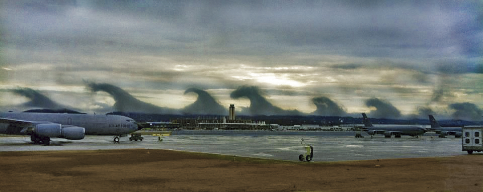
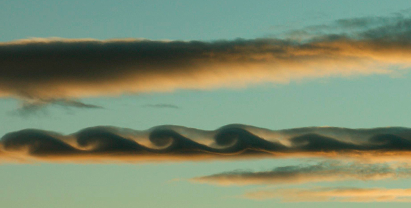
- Fig1_7a and Fig1_7b:
Characteristic Kelvin–Helmholtz instabilities in stormy clouds spotted at the
Birmingham–Shuttlesworth International Airport (USA) in December 2011 (Fig1_7a)
and round Sagunt (Valencia, Spain; Fig1_7b).
Credits: (a) WBMA–TV, Birmingham (Alabama, USA) and (b) Minerva Gracia; reproduced with permission.
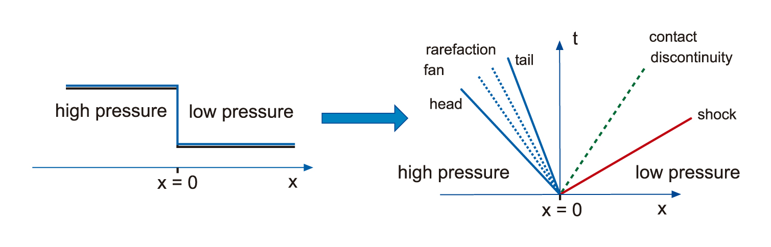
- Fig1_9b:
Diagram depicting the different types of discontinuities driven by a sharp pressure jump in a shock tube.
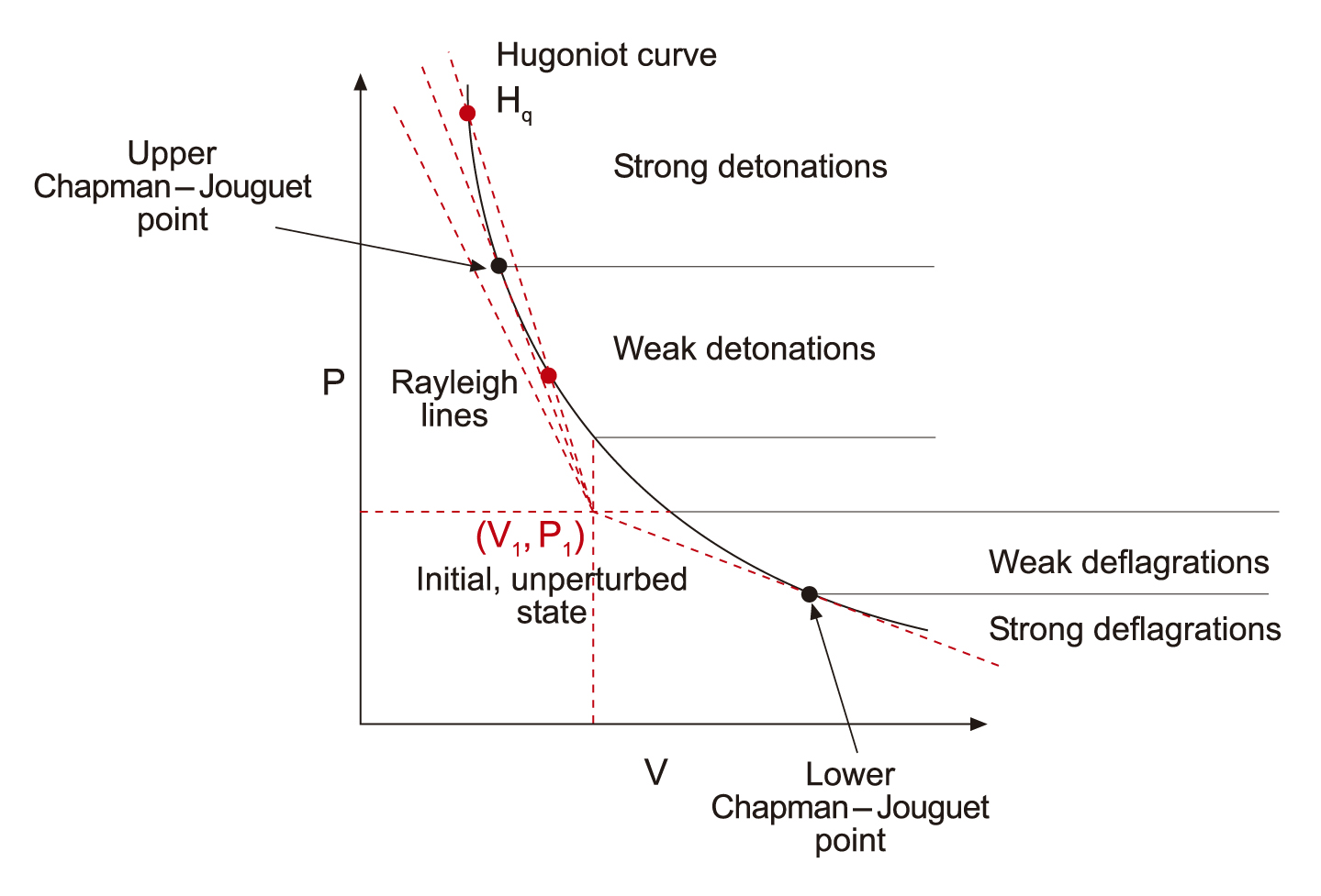
- Fig1_10a and Fig1_10b:
(Fig1_10a) The loci of all possible final states of a fluid after the passage of a combustion
front. (Fig1_10b) Final states reached through weak/strong deflagrations and detonations.
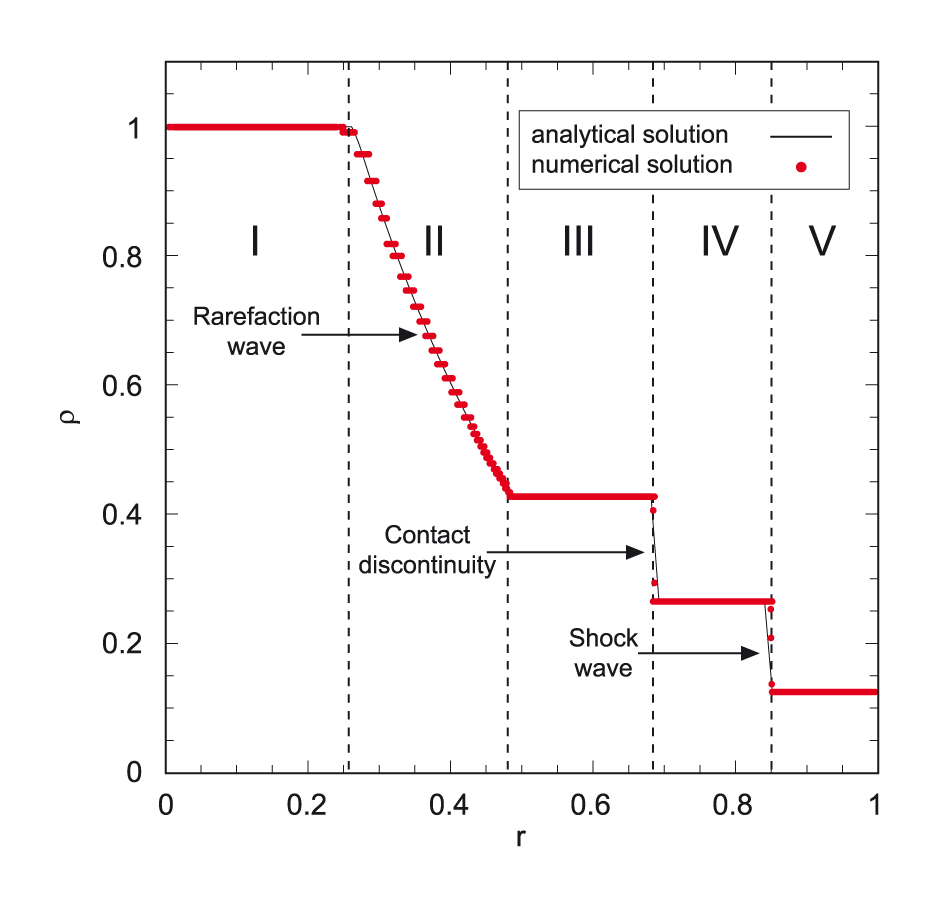
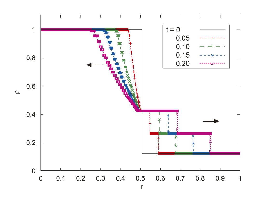
- Fig1_14a and Fig1_14b:
(Fig1_14a) Density profile at t = 0.2, in Sod’s shock tube problem, as computed with the FLASH
code. The plot displays the five distinct regions predicted theoretically, as well as the formation
of a rarefaction wave, a shock wave, and a contact discontinuity.
(Fig1_14b) Density profiles at times t = 0, 0.05, 0.1, 0.15, and 0.2 units, in Sod’s shock tube problem.
- Fig1_15:
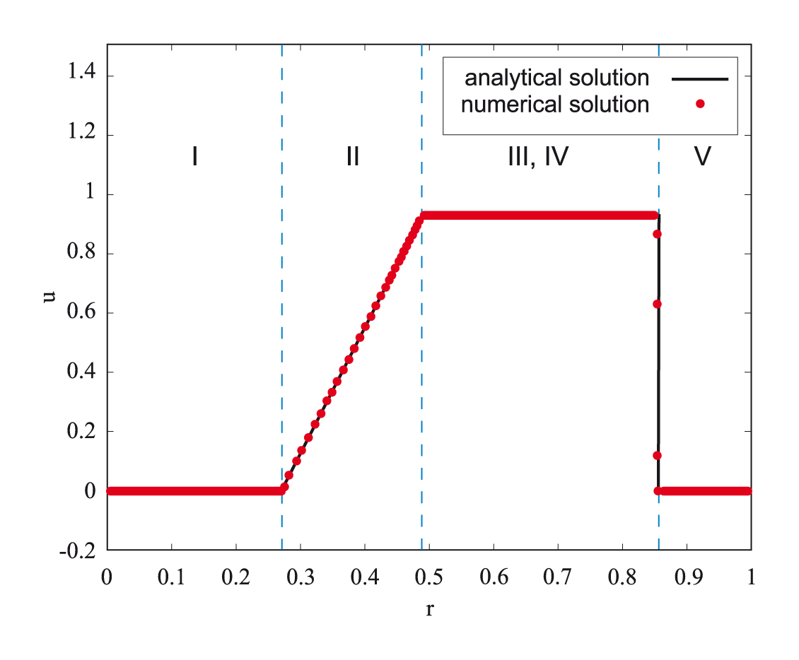
Comparison between the numerical velocity profile at t = 0.2 units and the analytical
solution in Sod’s shock tube problem.
- Fig1_16:
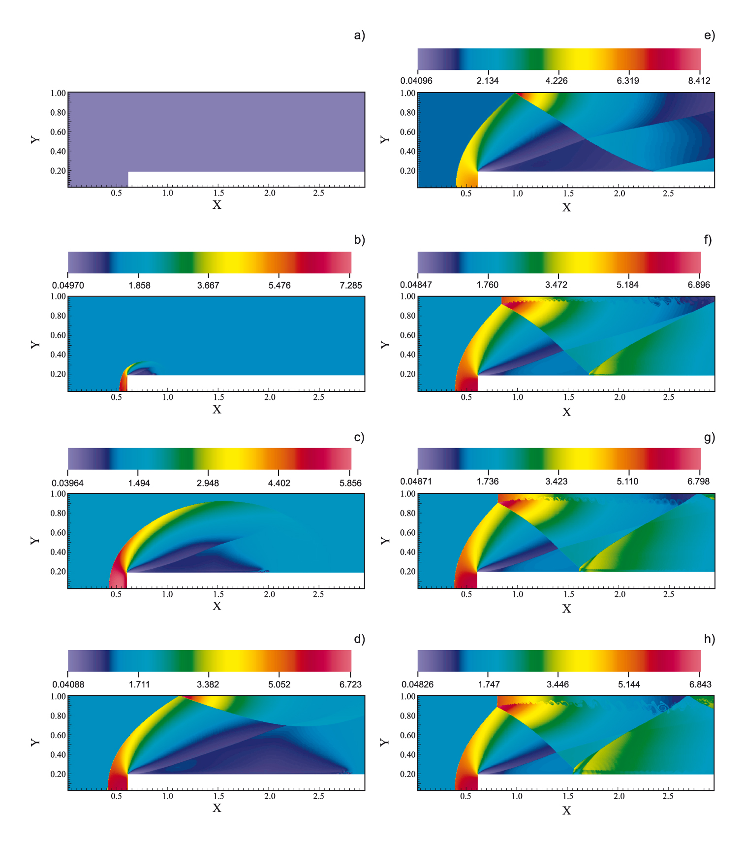
Evolution of the density field in Emery’s wind tunnel test, at times 0 (panel a), 0.1 (b), 0.5
(c), 0.8 (d), 1.3 (e), 2.6 (f), 3.3 (g), and 4 (h).
- Fig1_17a and Fig1_17b:
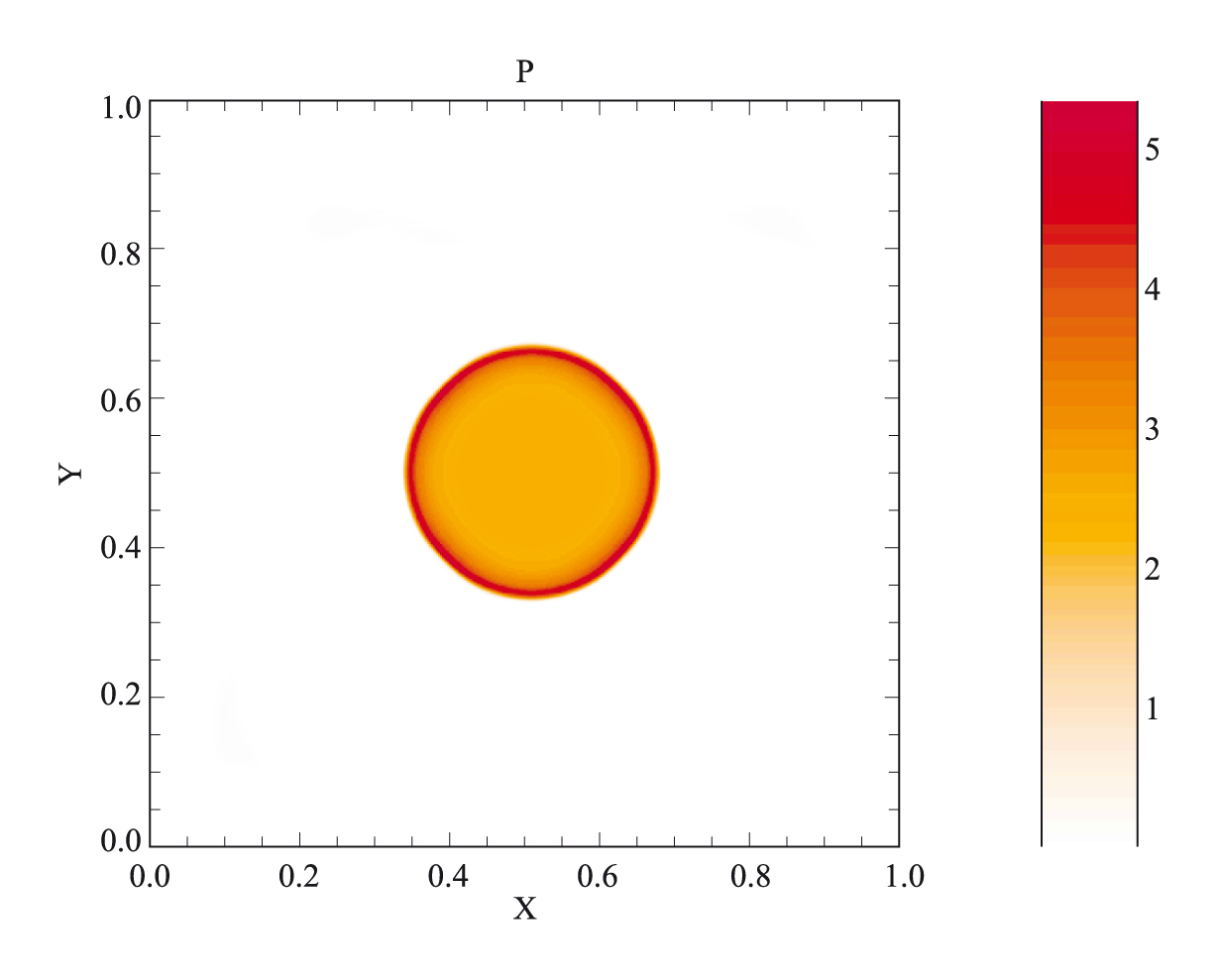
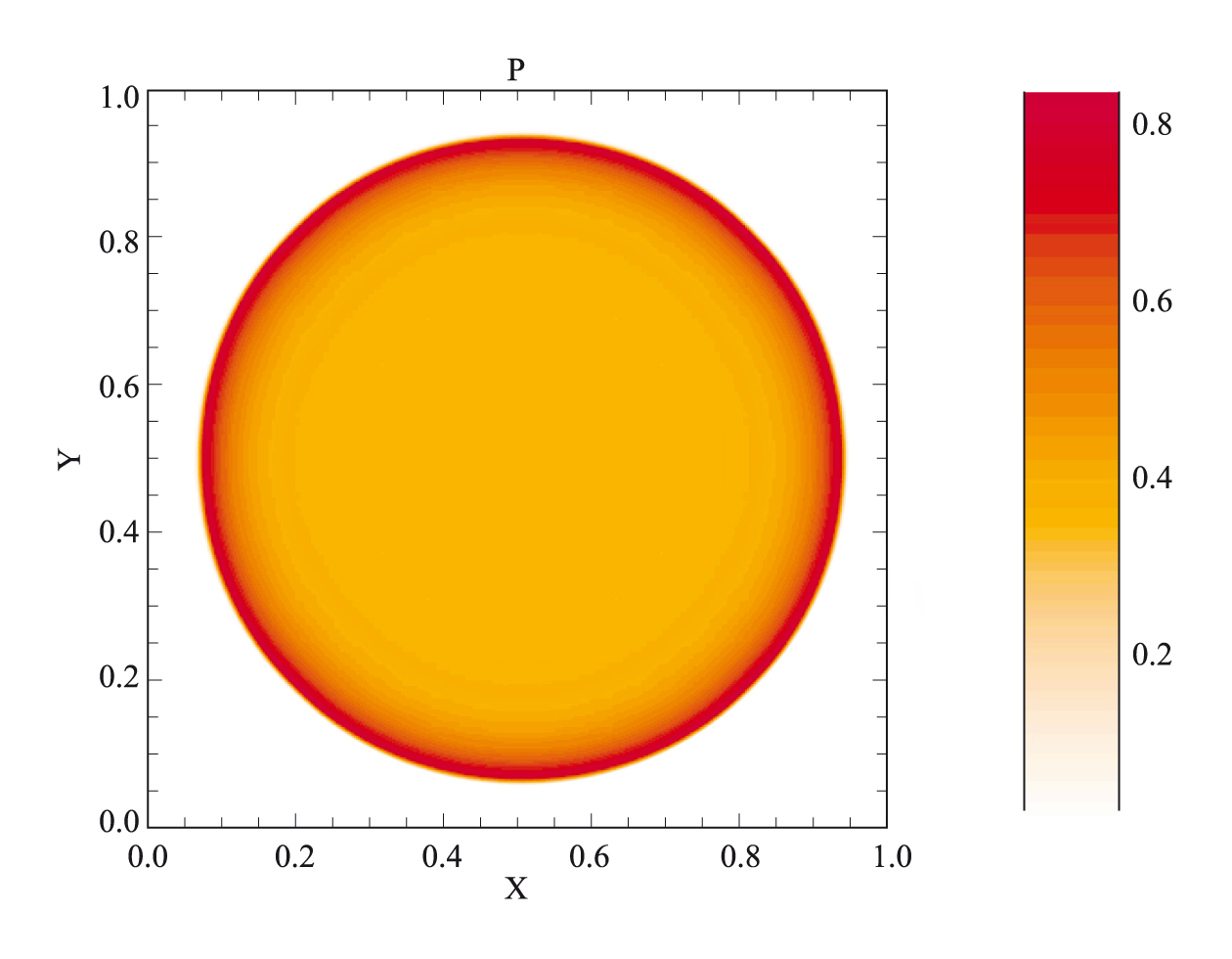
Snapshots of the pressure at (Fig1_17a) t = 0.03 and (Fig1_17b) 0.21 units, in Sedov’s blast
wave problem, showing that the spherical symmetry of the blast wave is preserved
as the detonation sweeps the computational domain.
- Fig1_18:
Comparison between the analytical pressure and the numerical value at t = 0.27
units, in Sedov’s blast wave problem.
- Fig1_19:
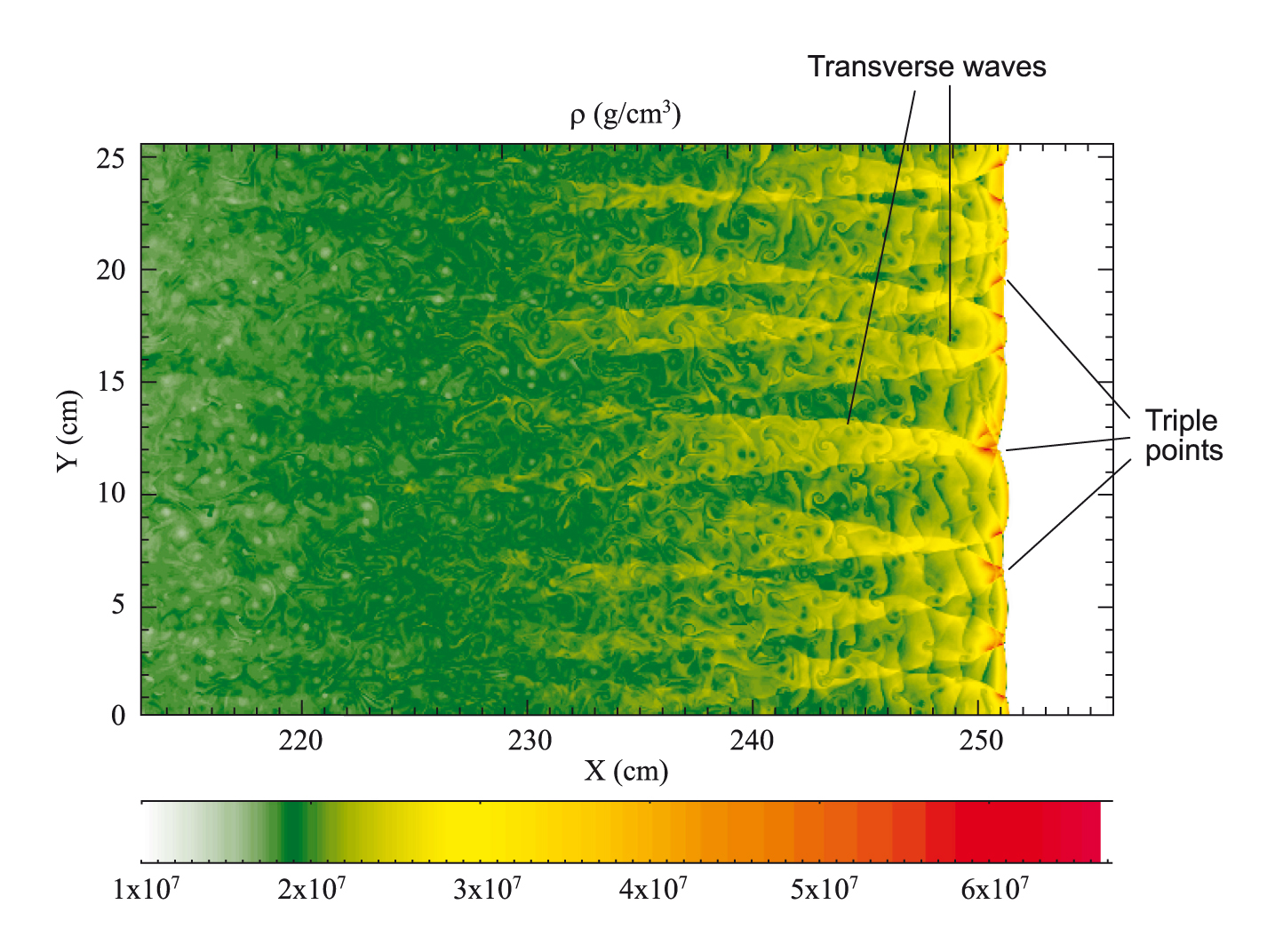
Snapshot of the density field at t = 185 ns, in the cellular problem. Incident shock
waves, triple points, and transverse waves can be identified, with a postshock structure
extending about 20 cm behind the front.
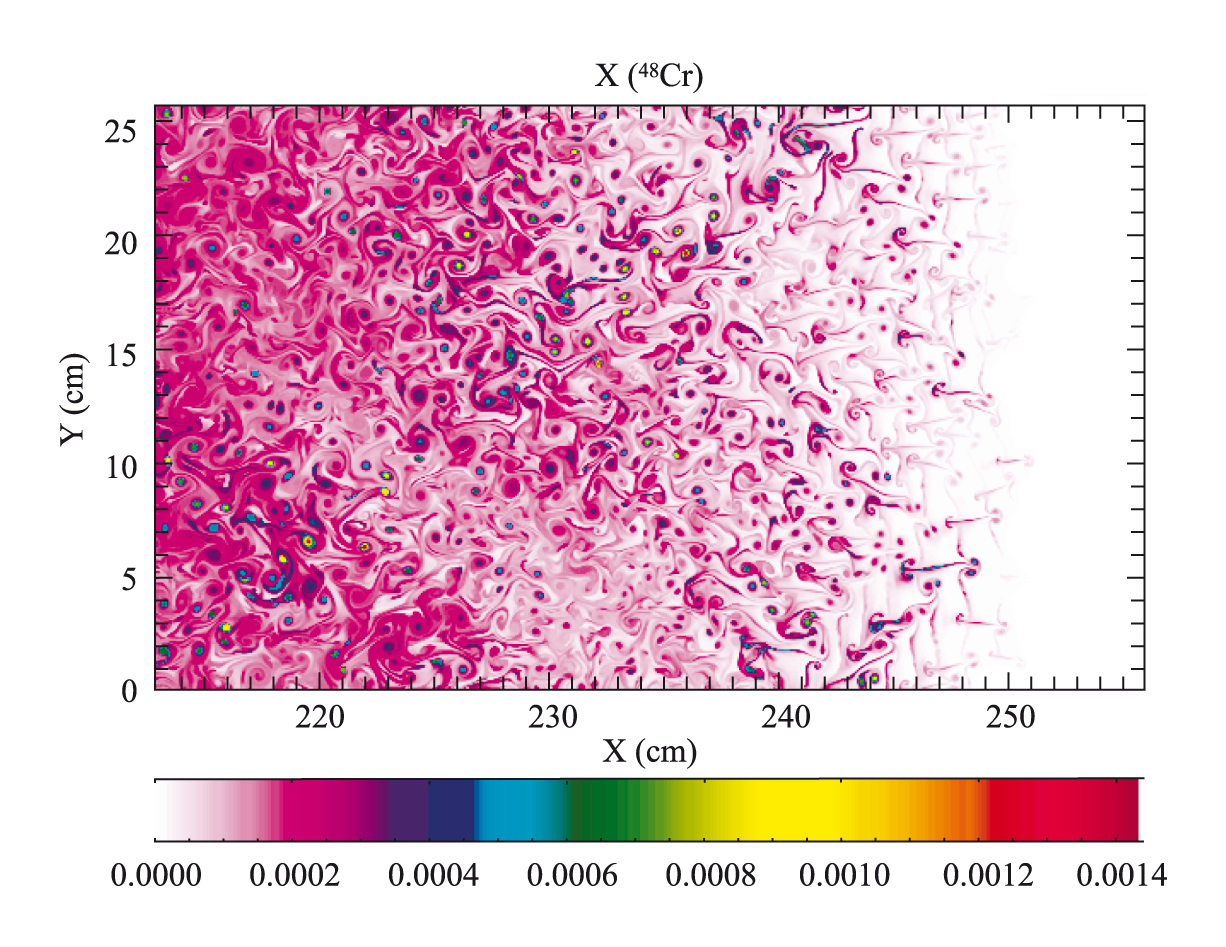
- Fig1_20a and Fig1_20b:
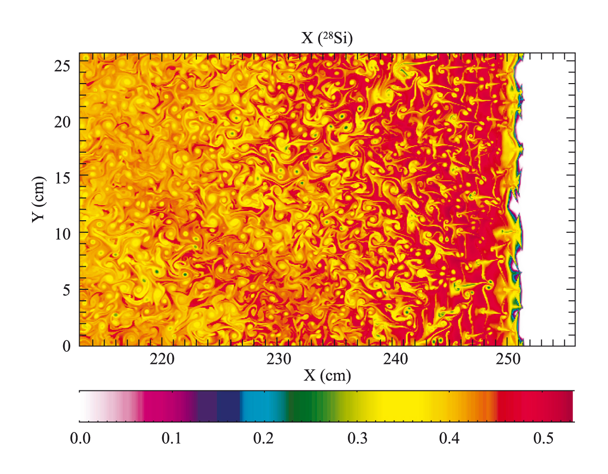
Distribution of 28Si and 48Cr in mass fractions at t = 185 ns in the cellular problem, showing
the onset of Kelvin–Helmholtz instabilities. Note that while 28Si increases from left to right,
the abundance of 48Cr decreases from left to right.
- Movie_Sod_test:
Time evolution of the density profile in the Sod's shock tube test.
- Movie_Wind_Tunnel_test:
Time evolution of the density in Emery's wind tunnel test.
- Movie_Sedov_test:
Time evolution of the pressure in Sedov’s blast wave test
[Movie in preparation].
- Movie_Cellular_D_test:
Time evolution of the density profile in the cellular problem
[Movie in preparation].
- Movie_Cellular_28Si:
Time evolution of the 28Si abundance in the cellular problem
[Movie in preparation].
- Movie_Cellular_48Cr:
Time evolution of the 48Cr abundance in the cellular problem
[Movie in preparation].
Chapter 2: Nuclear Physics
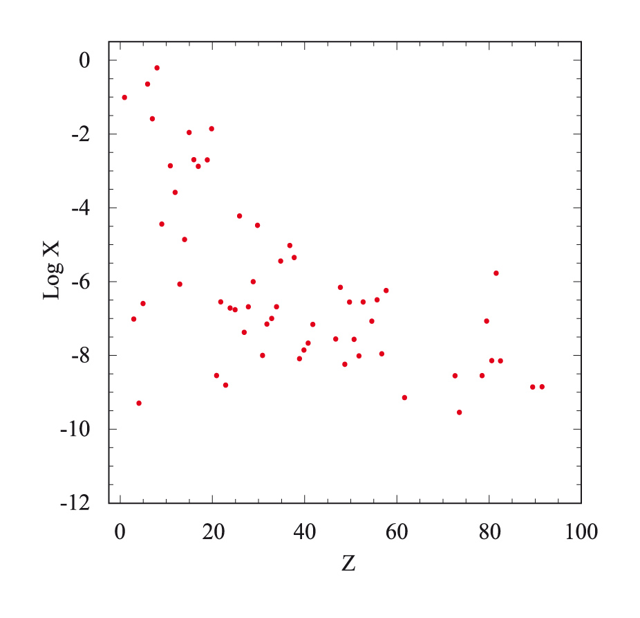
- Fig2_1a:
Elemental composition of the primitive Universe after Big Bang nucleosynthesis,
in mass fractions.
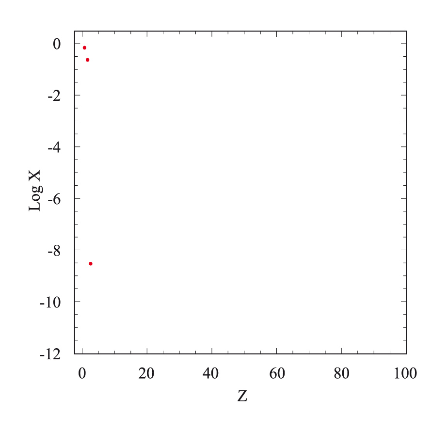
- Fig2_1b:
Elemental composition of the human body, in mass fractions, based on data from J.
Emnsley (1998).
- Fig2_2:
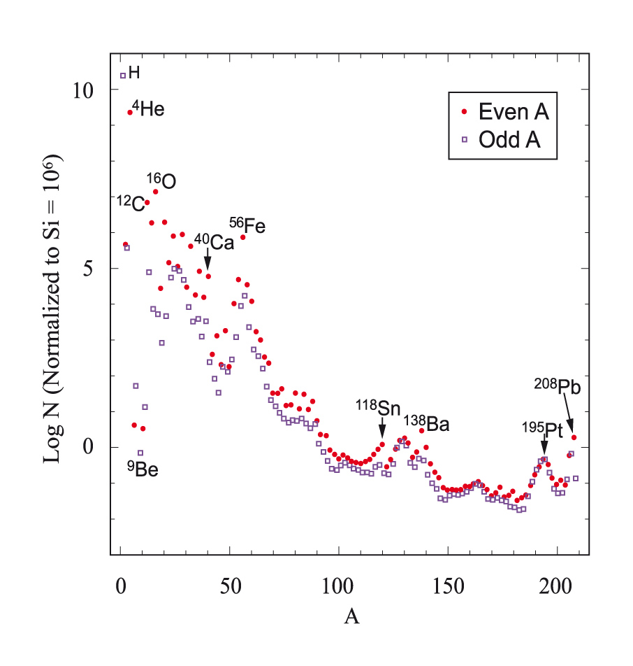
Solar System isotopic abundances versus mass number, based on data from K. Lodders (2003).
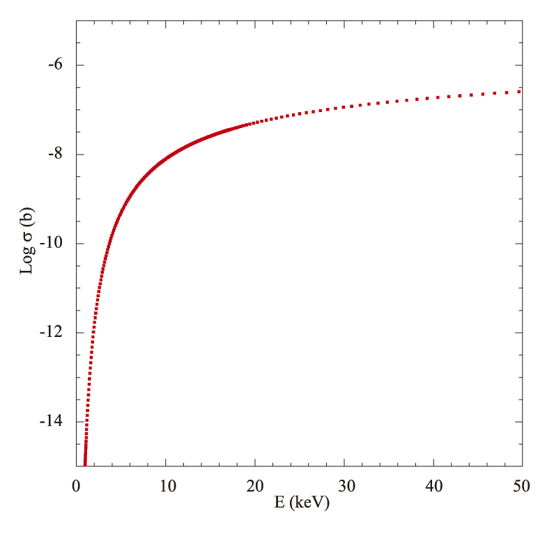
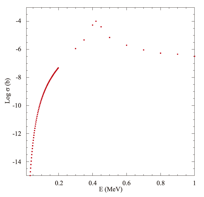
- Fig2_6a and Fig2_6b:
Experimental cross-section of the reactions d(p, γ)3He (Fig2_6a) and
12C(p, γ)13N
(Fig2_6b). Data courtesy of S. Goriely, based on the NACRE II compilation.
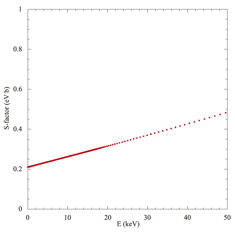
- Fig2_7:
Astrophysical S-factor for the reaction d(p, γ)3He.
Data courtesy of S. Goriely, based on the NACRE II compilation.
- Fig2_9:
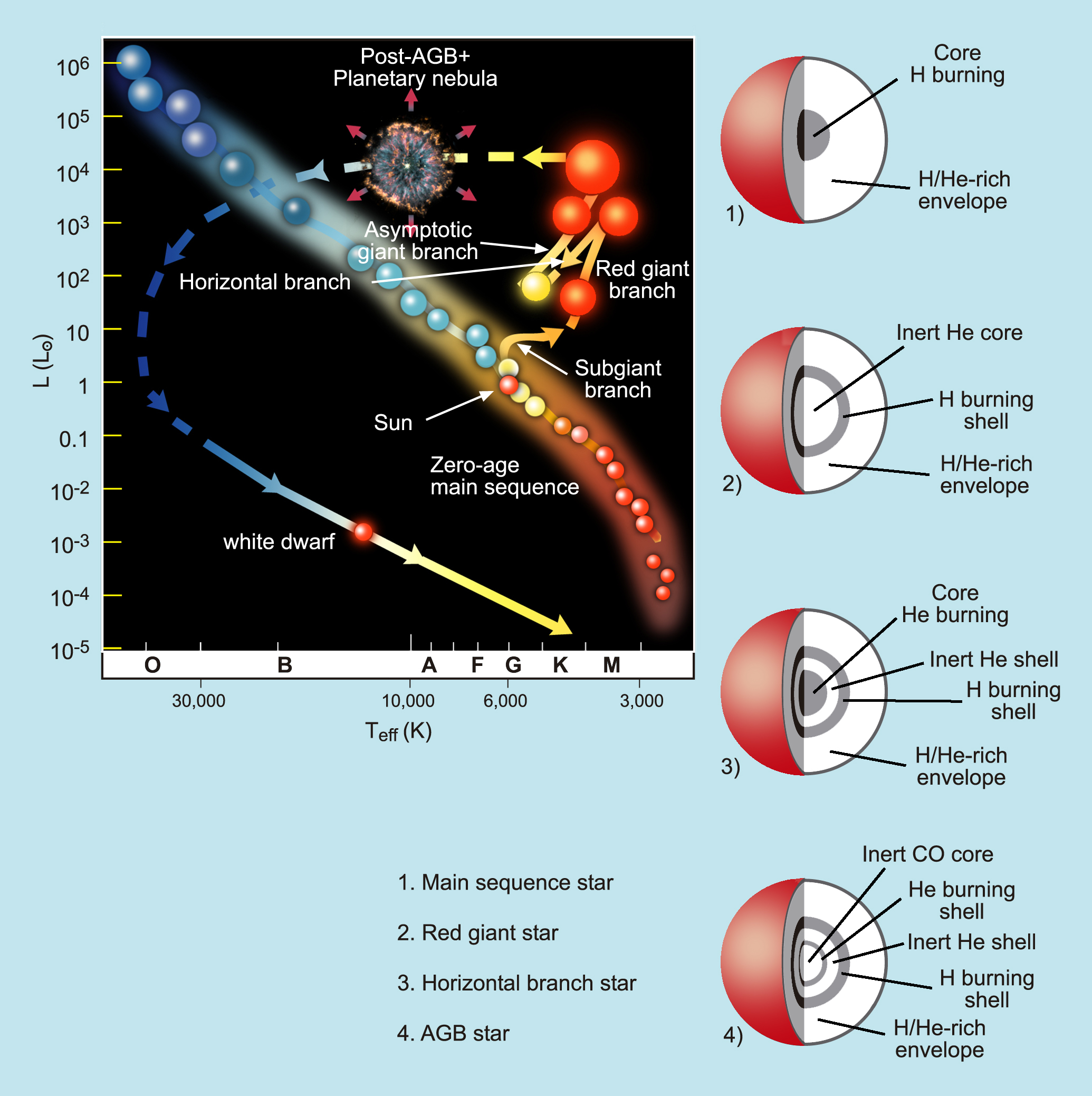
Evolution of the Sun in an H–R diagram, from core H-burning to the white dwarf stage. The
life of any star begins with core H-fusion (sphere 1), while occupying a characteristic location
on the diagram: the main sequence. In a star like the Sun, H will be depleted near the center
after 10 Gyr. Following recontraction, H will ignite in the shells that surround the He-rich
core, leading to a dramatic increase in size, approximately reaching the orbit of the
Earth. Its path along the H–R diagram will subsequently follow the subgiant and red giant
branches, while the Sun becomes a giant star (2). The temperature rise at the center during
recontraction will eventually lead to core He-ignition. Its evolution will continue through the
horizontal branch (3). After 1 Gyr, helium will be depleted at the center and double H- and
He-shell burning will set in. The Sun, by then a bright star (4), will climb the asymptotic
giant branch (AGB). The late stages will be characterized by a gentle ejection of the outer
layers at v = 50 - 100 km s-1, giving rise to a planetary nebula, while the inner, CO-rich 0.6
Msun of the Sun will smoothly evolve into a stable, white dwarf configuration.
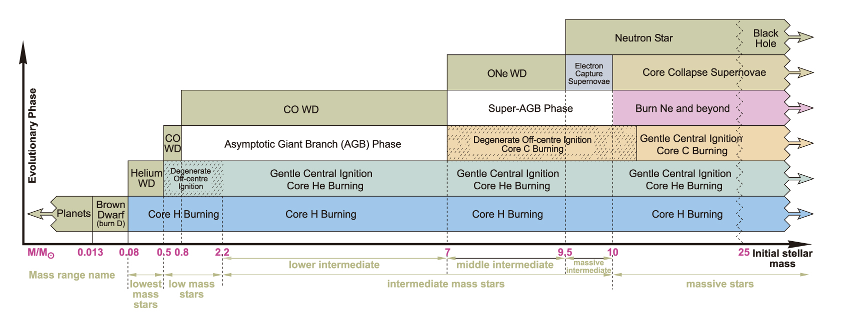
- Fig2_10:
Summary of the main burning stages and end products of stellar evolution as a function of
the stellar mass, based on solar metallicity models. Figure adapted from
A. Karakas and J. Lattanzio (2014); reproduced with permission.
- Fig2_11:
H-burning through the pp chains. According to the Standard Solar Model, the pp
chains proceed in the solar interior through chain 1 about 85% of the times, 15% through
chain 2, and only 0.02% through chain 3. The horizontal arrow that connects H and d
corresponds to p(p, e+ν)d, while those that connect 7Li and 8Be
with 4He correspond to
the decays 7Li(p, α)α and 8Be(α)α, respectively.
- Fig2_12:
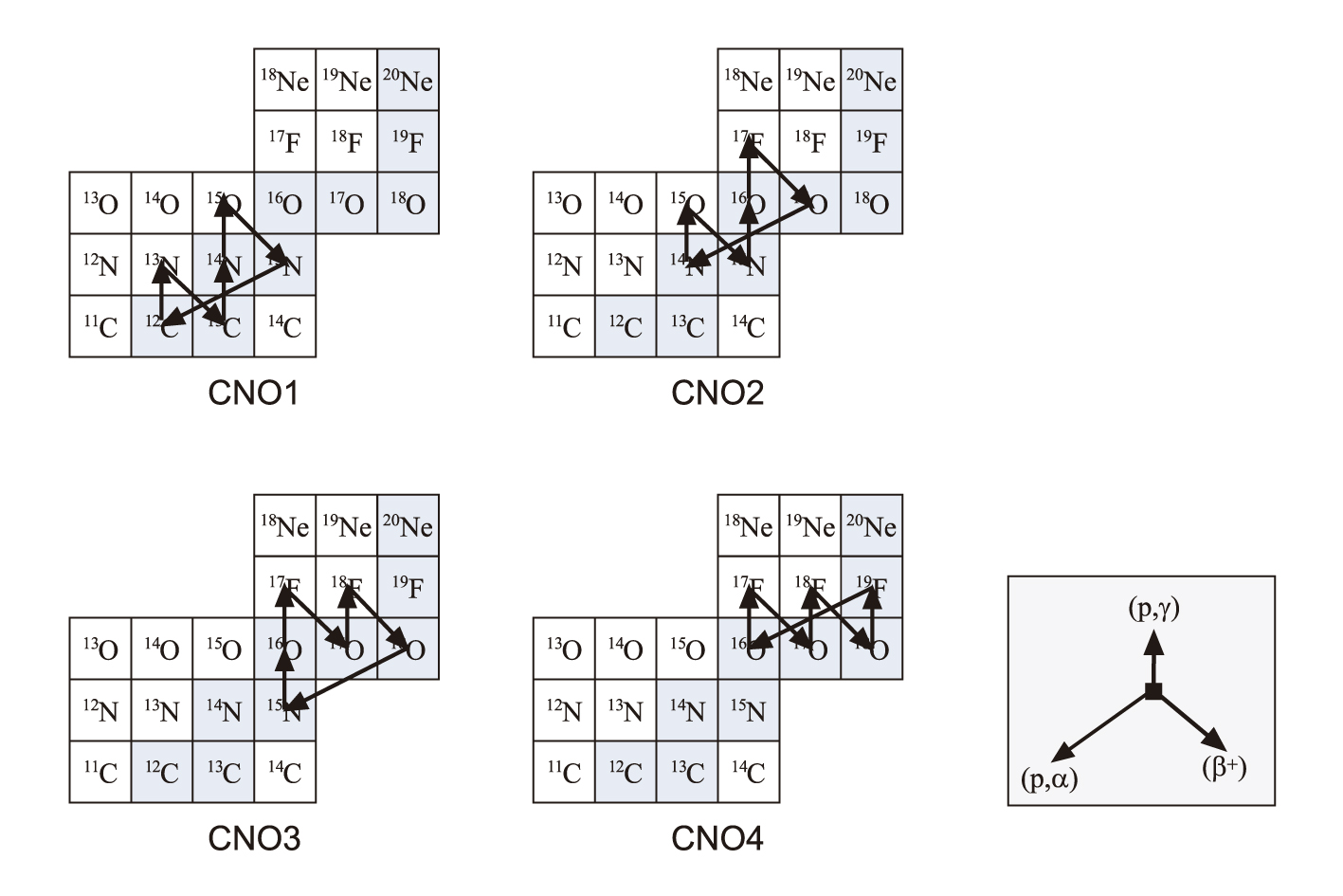
H-burning through the cold CNO cycles.
- Fig2_13:
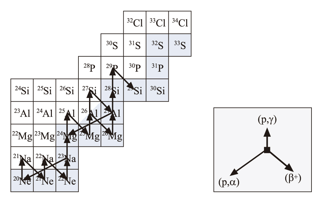
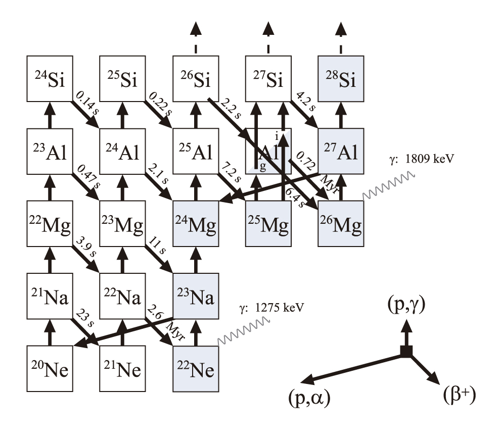
H-burning in the NeNa–MgAl mass region. Two different states for 26Al, the ground state and a short-lived,
isomeric state, are actually distinguished.
- Fig2_14:
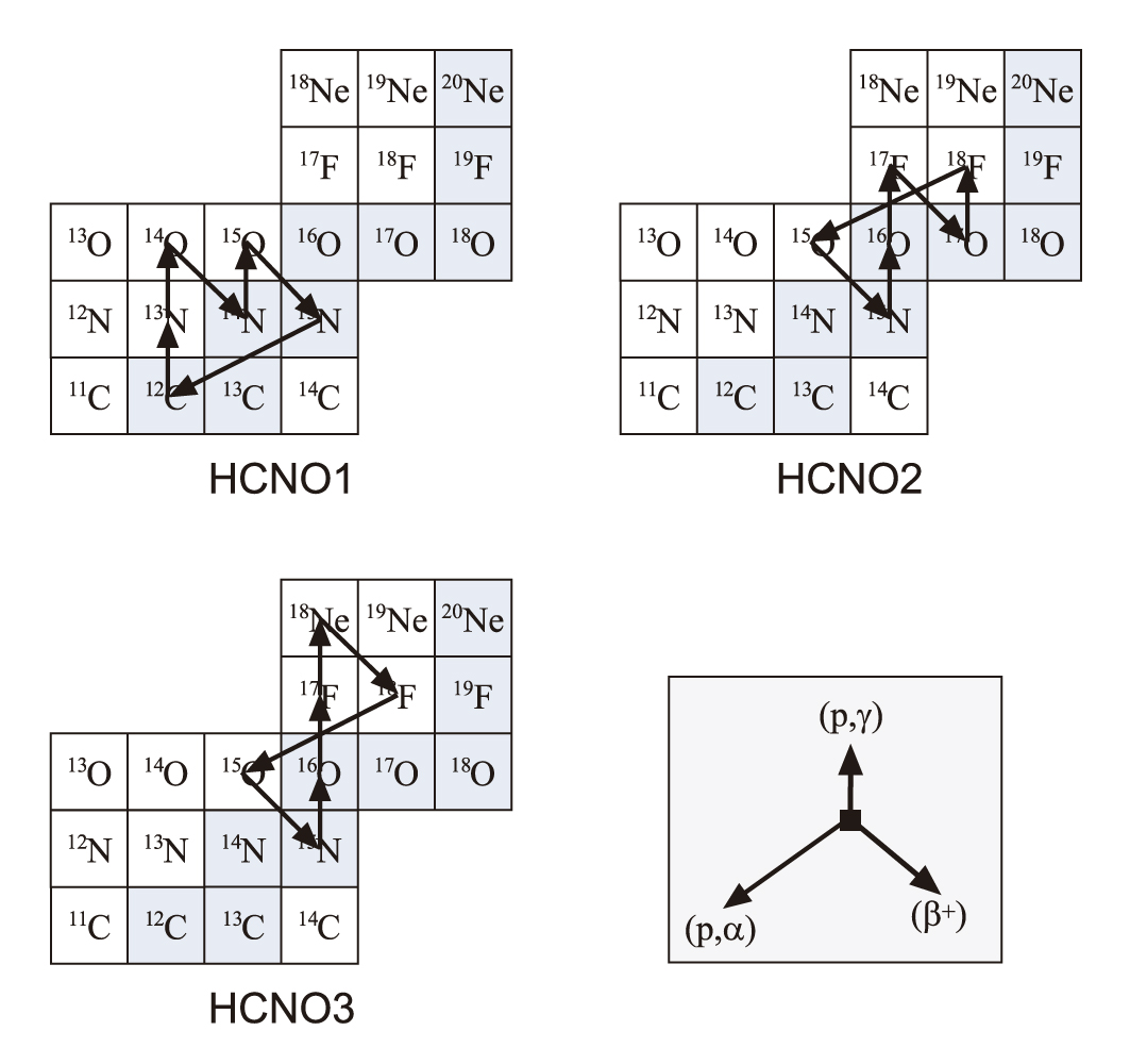
Explosive hydrogen burning through the hot CNO cycles.
- Fig2_15:
Explosive H-burning reactions in the A ≥ 20 mass region.
- Fig2_16a and Fig2_16b:
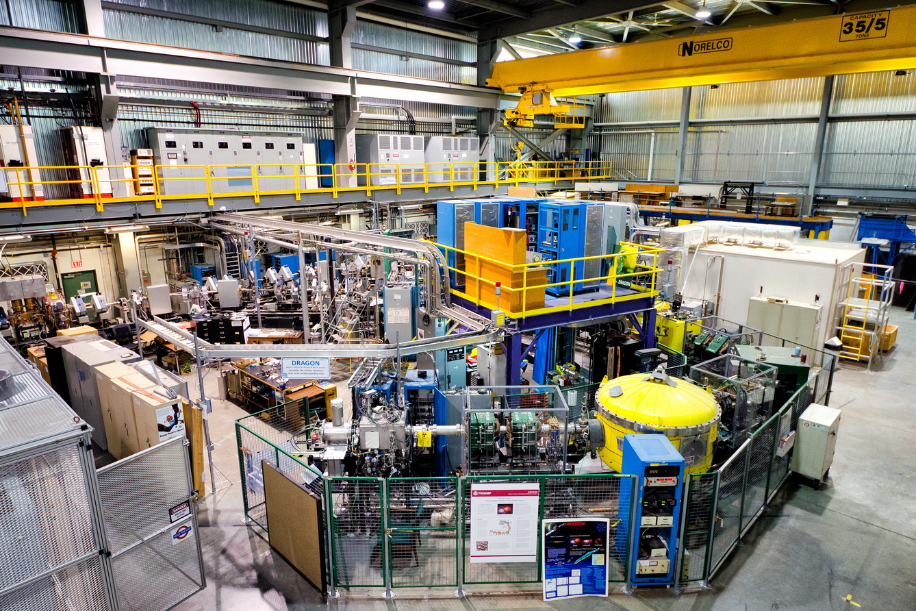
DRAGON, a recoil mass separator for the study of nuclear reactions of astrophysical
interest, located in the ISAC facility at TRIUMF (Vancouver). Image courtesy of Steven
Oates.
Chapter 3: Cosmochemistry and Presolar Grains
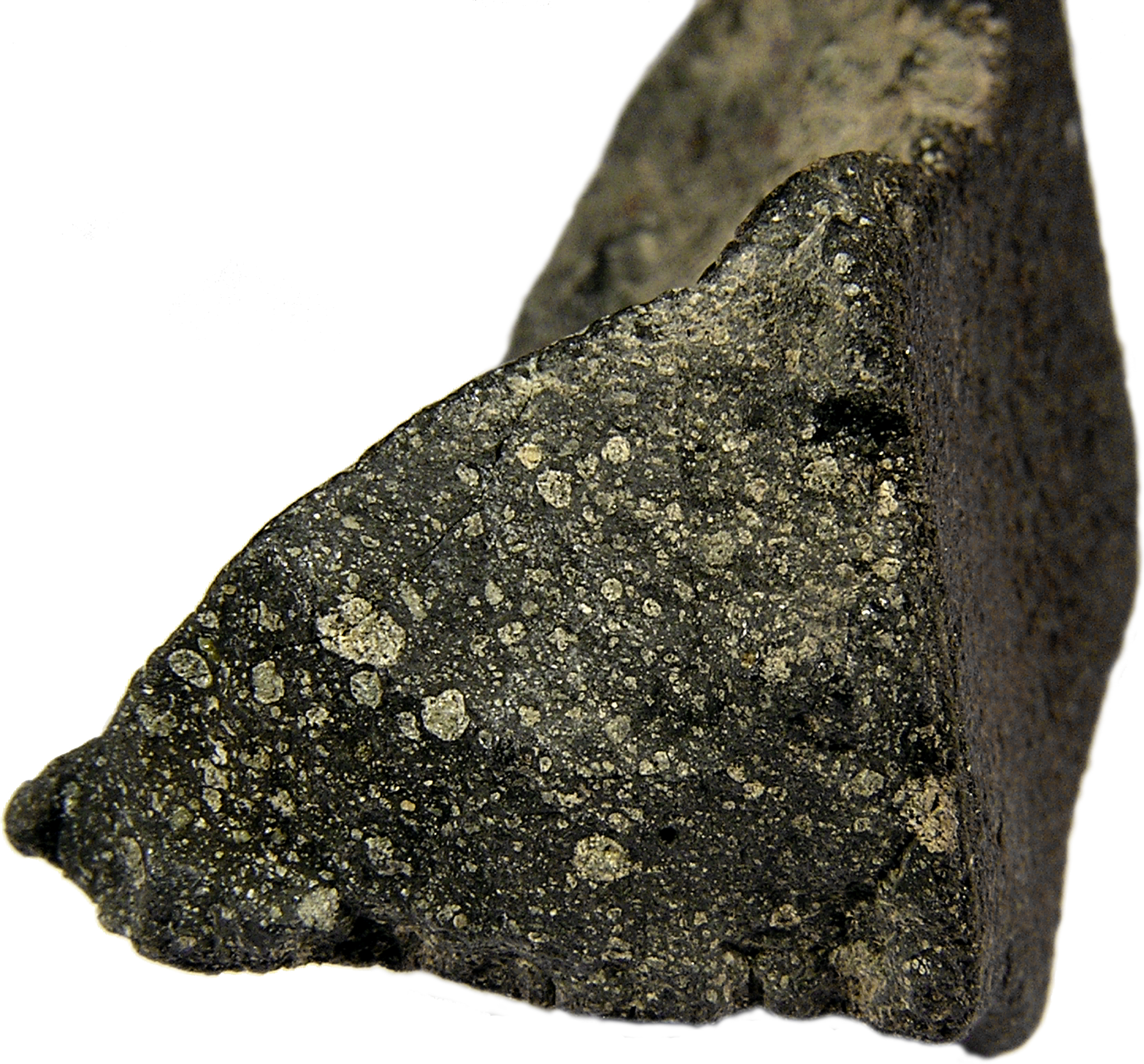
- Fig3_1:
Fragment of the Murchison meteorite, a carbonaceous chondrite that fell in Australia
on september 28, 1969. Credit: Meteorites Australia; reproduced with permission.
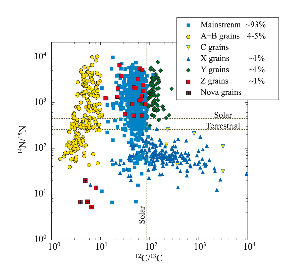
- Fig3_3:
Carbon and nitrogen isotopic ratios for the different SiC grain populations. Figure courtesy of E. Zinner.
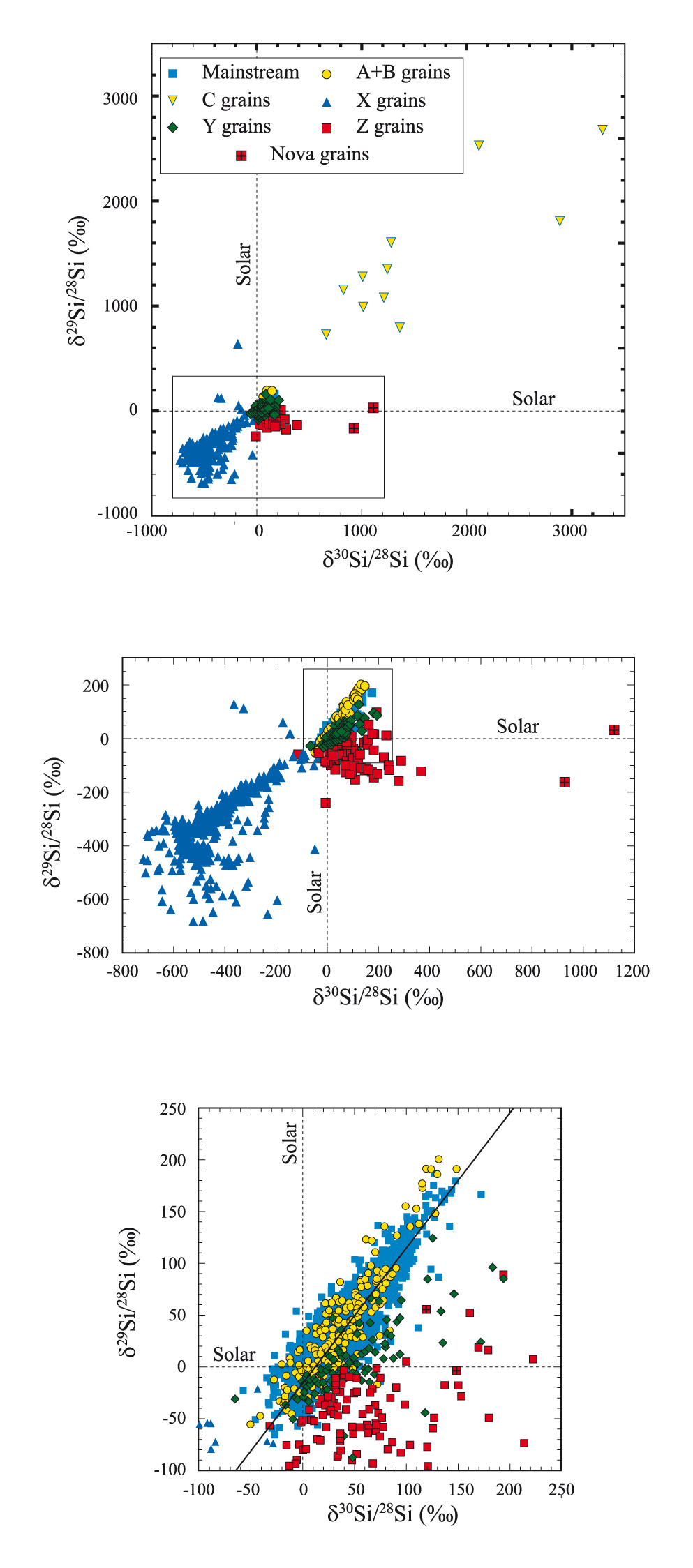
- Fig3_4:
Silicon isotopic ratios measured in presolar SiC grains, expressed as
delta values, or deviations from the solar isotopic ratios in permil. Figure courtesy of E. Zinner.
- Fig3_8a:
The Transmission Electron Microscope of the Center for Biotechnology of the
University of Nebraska–Lincoln, in the US. The device has a resolution up to
0.5 nm, under ideal conditions. Image courtesy of the University of Nebraska–Lincoln, reproduced with permission.
- Fig3_9a:
Schematic view of the operation of a SIMS spectrometer.
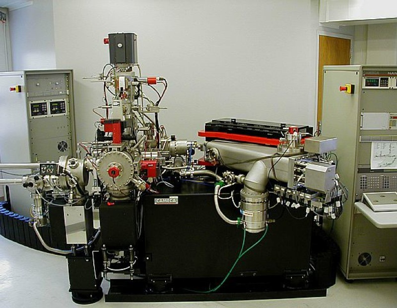
- Fig3_9b:
Photograph of NanoSIMS 50, the first of its kind, designed specifically for the study of presolar grains. This ion
microprobe, installed in the year 2000 at the Laboratory for Space Sciences of the Washington
University at St. Louis (USA), has an advanced multicollection system and achieves
a spatial resolution of about 100 nm. Figure courtesy of the Laboratory for Space Sciences
(WUST); reproduced with permission.
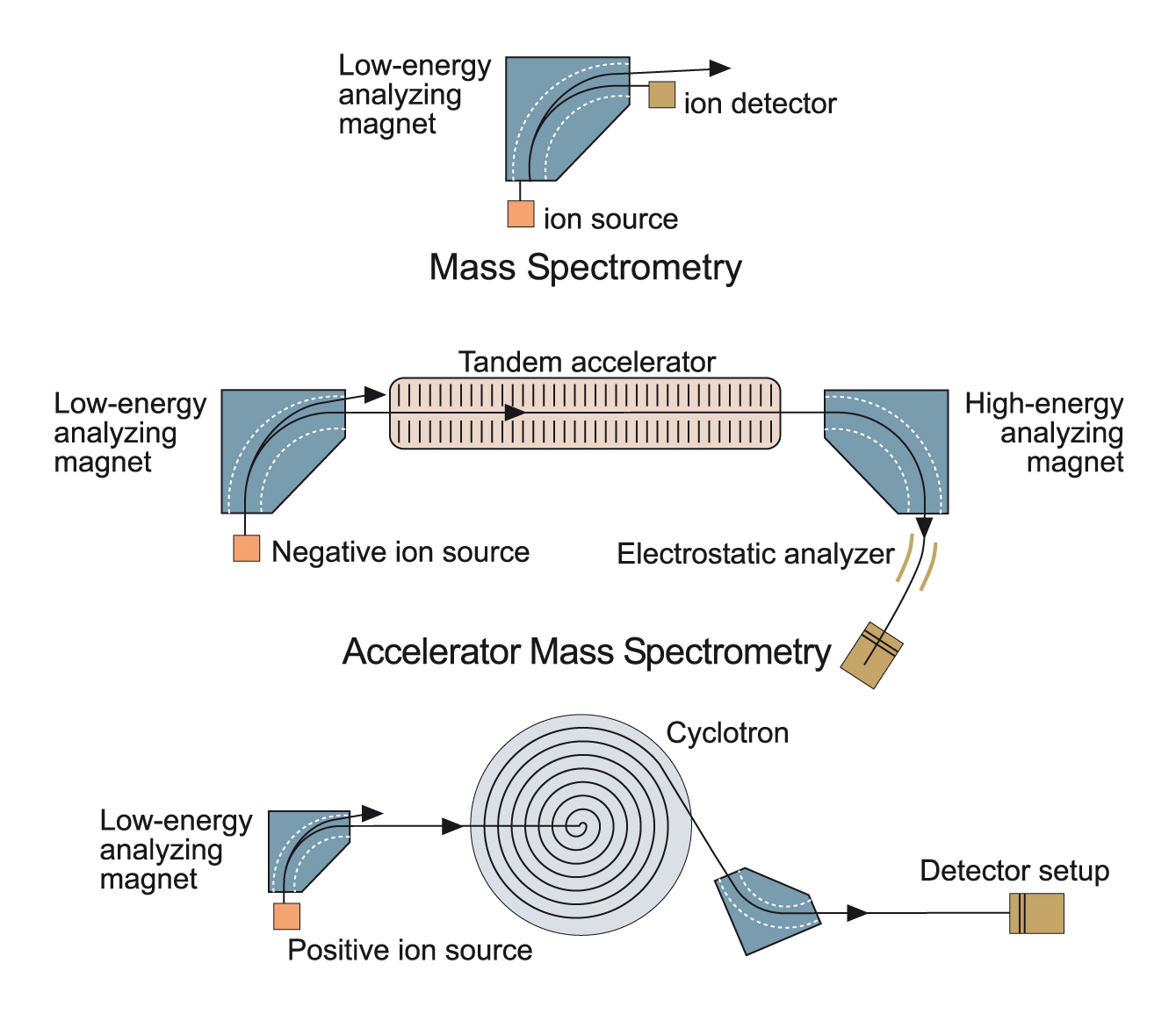
- Fig3_11a:
Accelerator Mass Spectroscopy (AMS) compared with standard Mass Spectroscopy. In AMS, secondary ions
sputtered from the sample are accelerated by means of a Tandem accelerator or a cyclotron.
- Fig3_11b:
A section of the AMS facility at the Maier–Leibnitz–Laboratory (TU Munich), in Garching, Germany,
showing the Tandem accelerator. Image courtesy of Shawn Bishop.
Chapter 4: Classical and Recurrent Novae
- Fig4_2:
Snapshots of the progress of a thermonuclear runaway in a nova outburs on
a 1.15 Msun CO white dwarf, calculated with the hydrodynamic code SHIVA.
- Fig4_3b:
Velocity field of a 2D simulation (1 km × 1 km) of mixing at the core-envelope interface
during a nova outburst on a 1 Msun CO white dwarf.
Calculations were performed with the PROMETHEUS code. Figure from
Kercek, Hillebrandt and Truran, reproduced with permission.
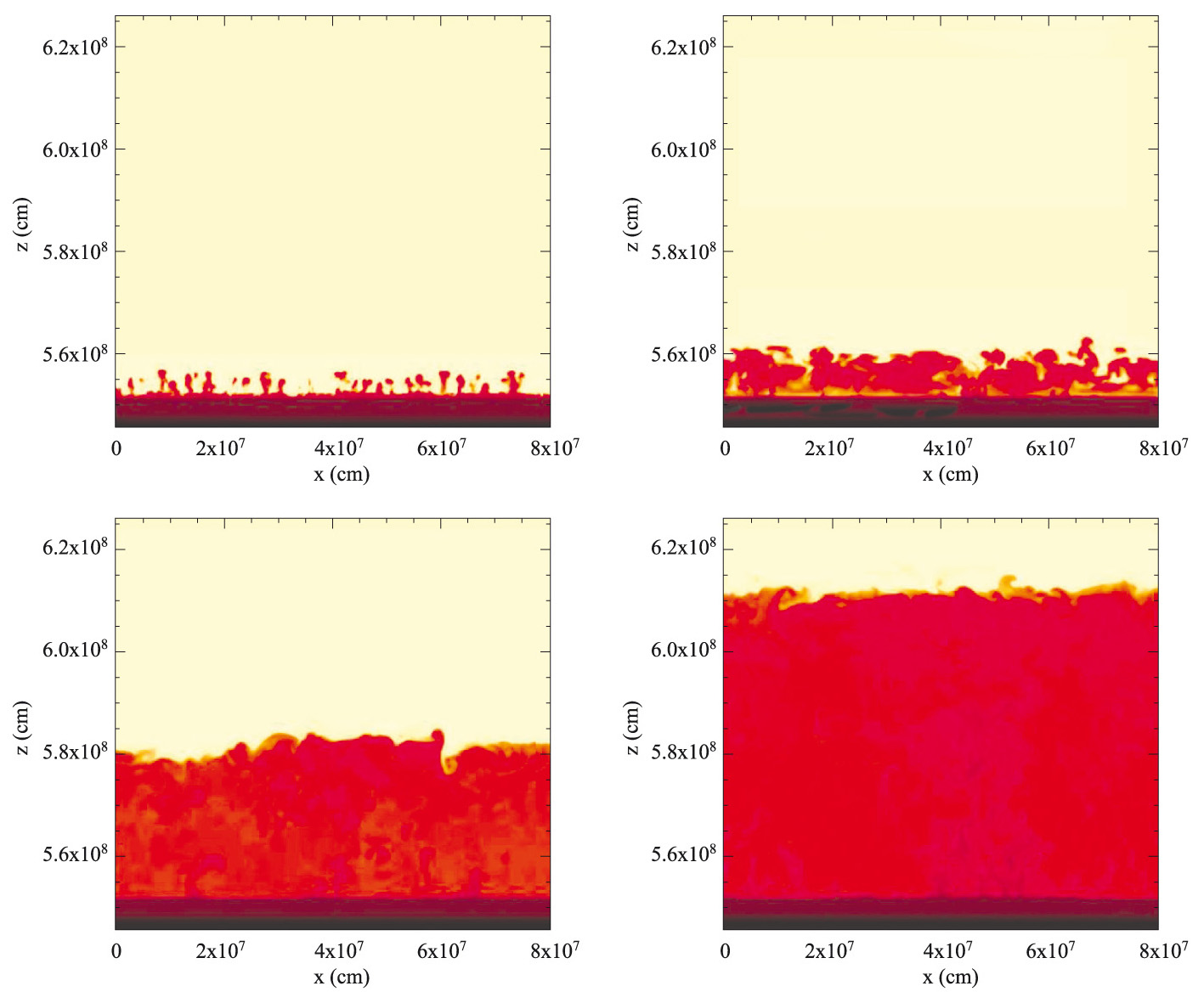
- Fig4_4:
Two-dimensional snapshots of the development of hydrodynamic instabilities,
in a 3-D simulation of mixing at the core-envelope interface during a
nova explosion, calculated with the hydrodynamic code FLASH.
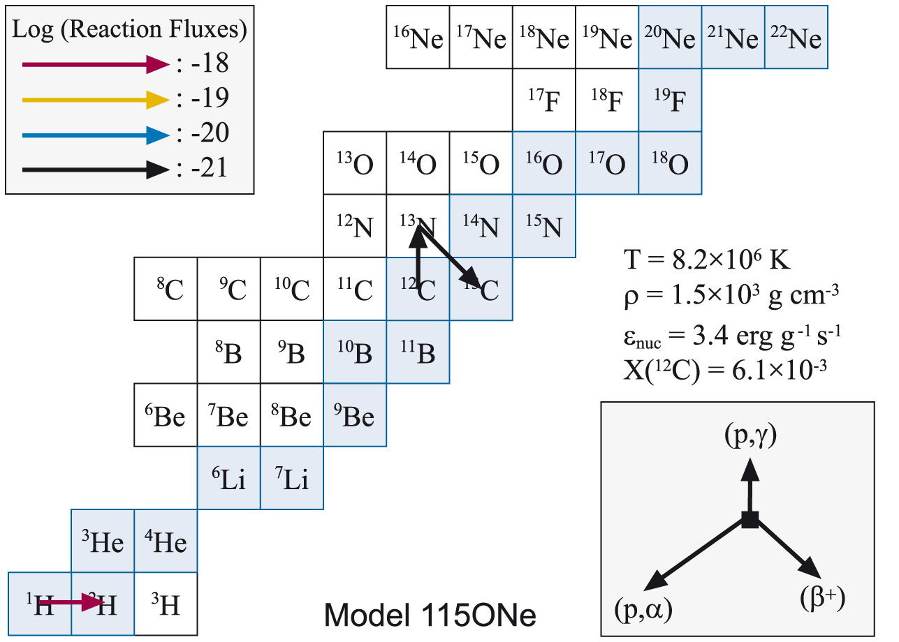
- Fig4_5a:
Main reaction fluxes at the innermost envelope shell for model 115ONe,
at the onset of accretion.
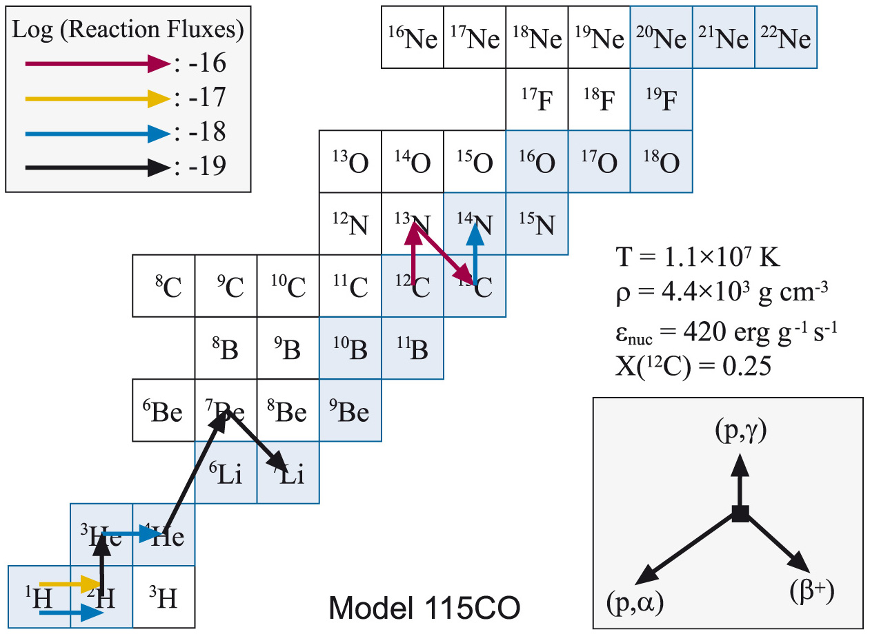
- Fig4_5b:
Main reaction fluxes at the innermost envelope shell for model 115CO,
at the onset of accretion.
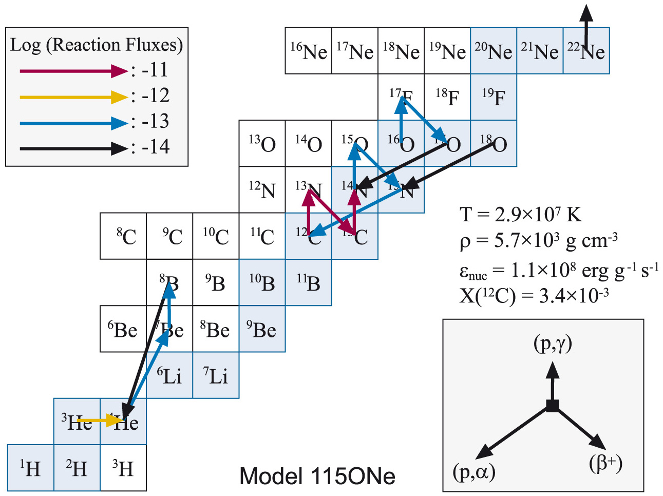
- Fig4_6a:
Main reaction fluxes at the innermost envelope shell for model 115ONe,
at T(base) = 1.1×10+7 K.
- Fig4_6b:
Main reaction fluxes at the innermost envelope shell for model 115CO,
at T(base) = 1.1×10+7 K.
- Fig4_7a:
Main reaction fluxes at the innermost envelope shell for model 115ONe,
at the end of the accretion stage.
- Fig4_7b:
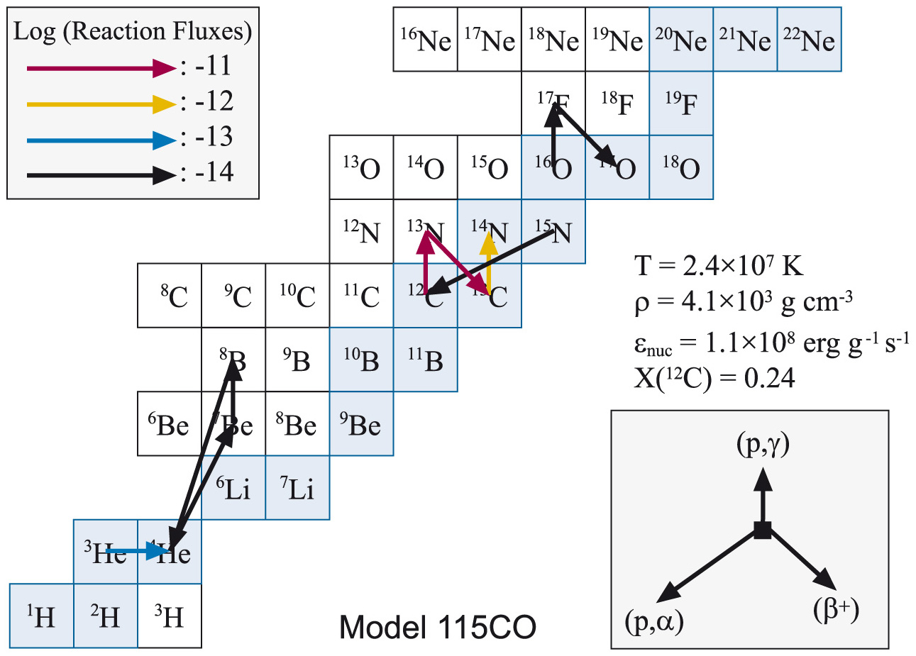
Main reaction fluxes at the innermost envelope shell for model 115CO,
at the end of the accretion stage.
- Fig4_8:
Main reaction fluxes at the innermost envelope shell for Model 115CO, at
peak temperature.
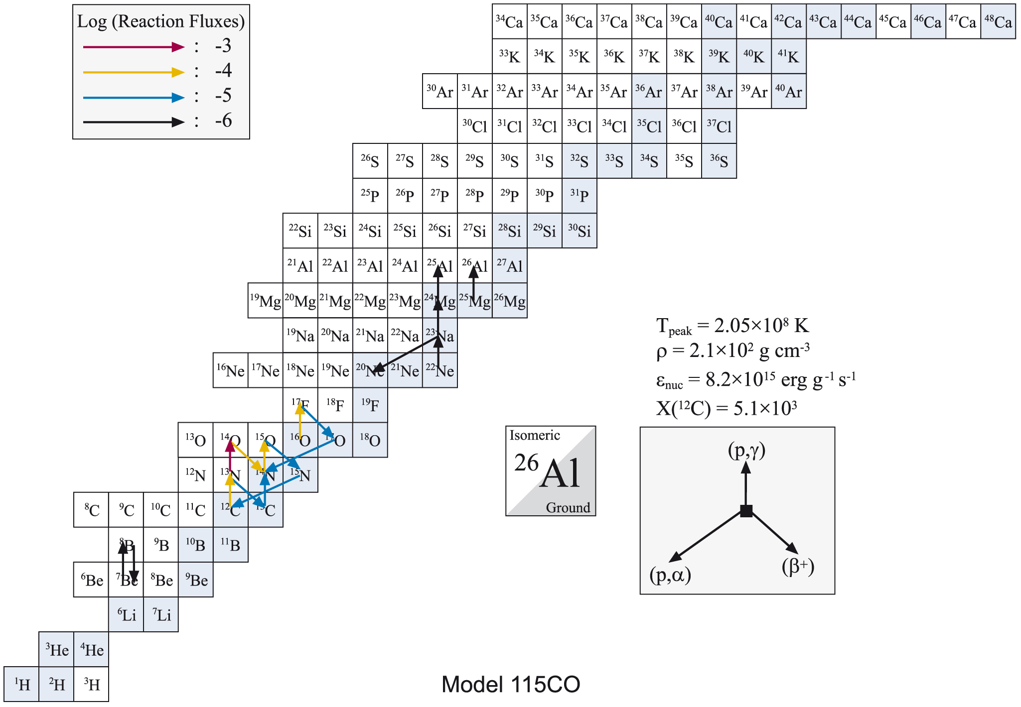
- Fig4_9:
Main reaction fluxes at the innermost envelope shell for Model 115ONe, at
peak temperature.
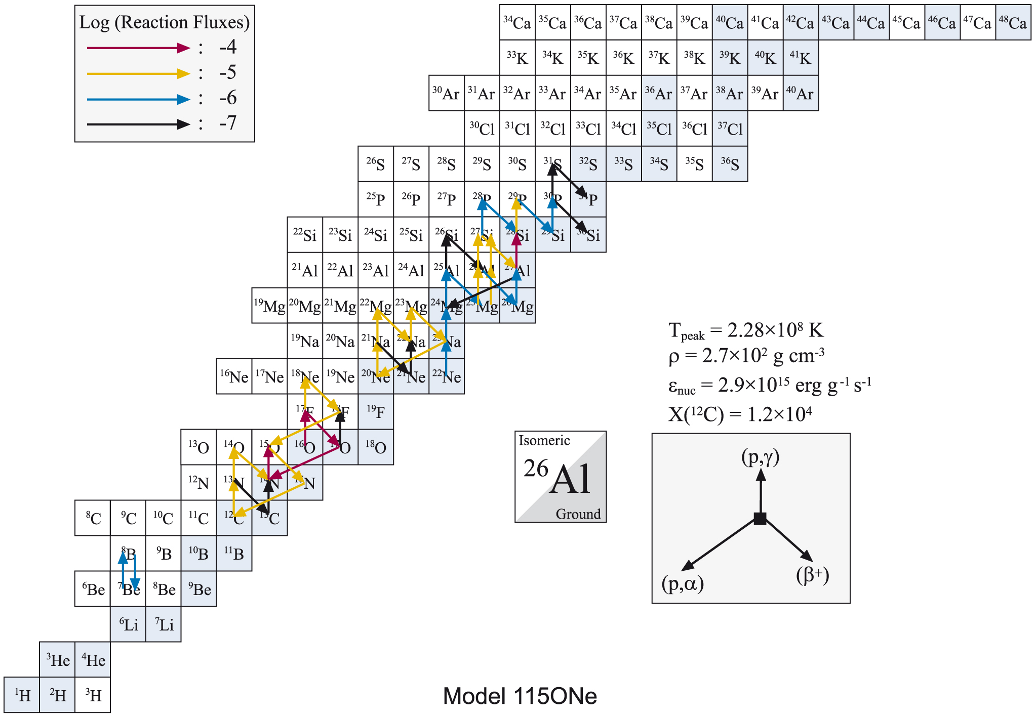
- Fig4_10:
Main reaction fluxes at the innermost envelope shell for Model 135ONe, at
peak temperature.
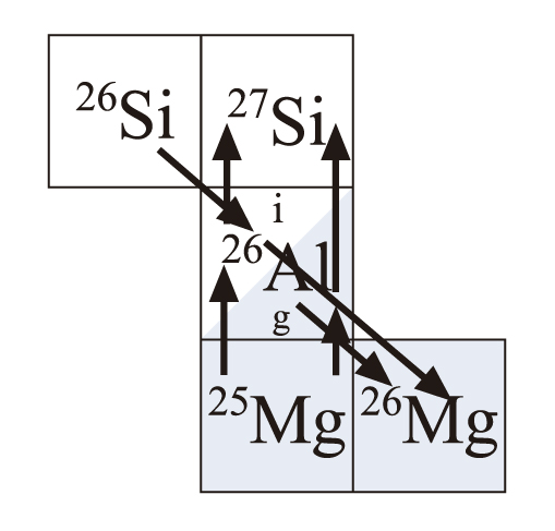
- Fig4_11:
Main nuclear interactions affecting 26Al ground (g) and isomeric (i)
states, for nova conditions.
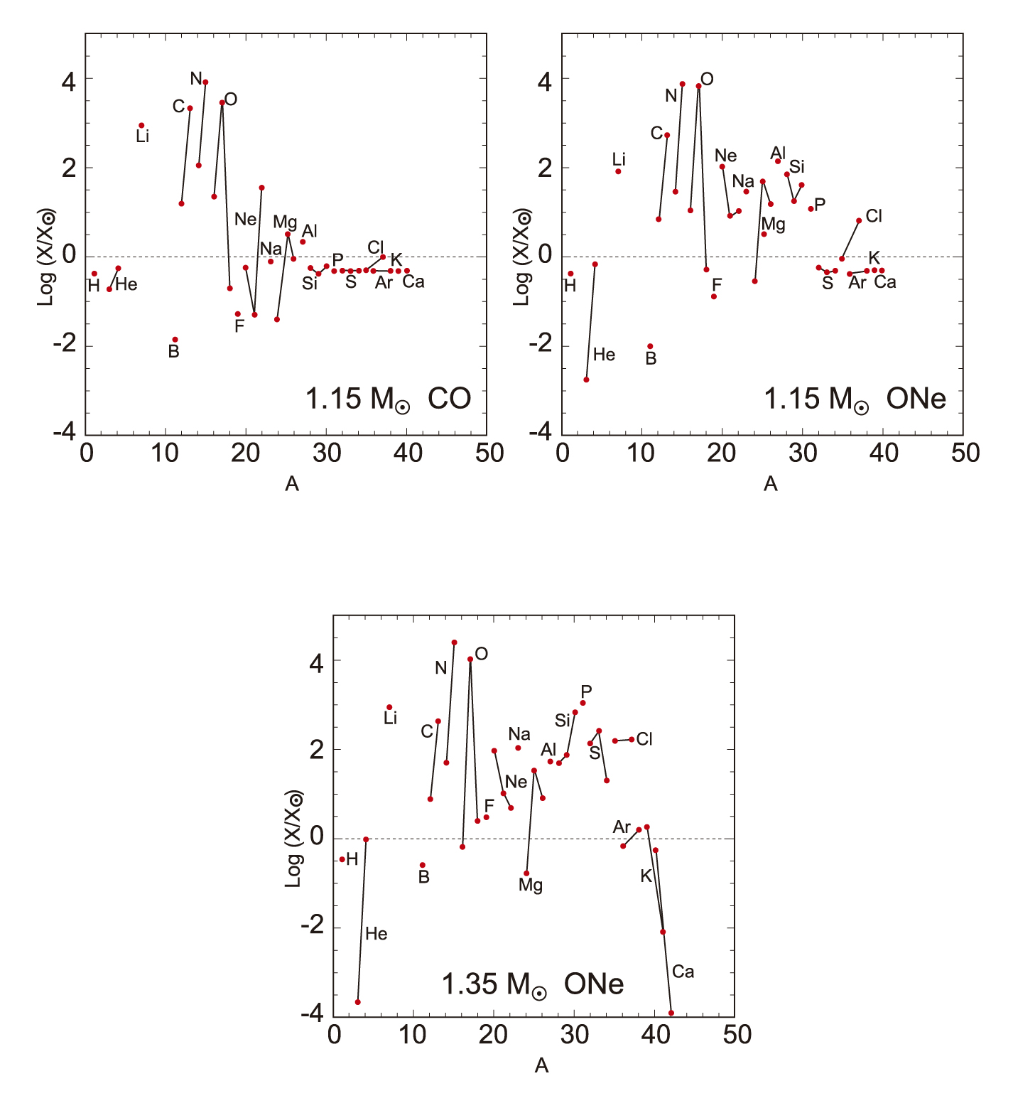
- Fig4_12:
Mean overproduction factors, relative to solar, in the ejecta of models 115CO (upper left
panel), 115ONe (upper right) and 135ONe (lower panel).
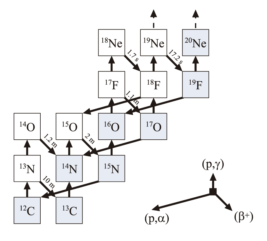
- Fig4_13:
Nuclear processes relevant for the synthesis of 18F in novae. Half-lifes of the
most important β+-decays are listed.
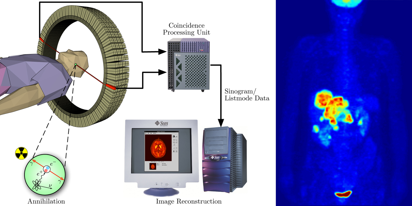
- Fig4_14:
Positron emission tomography (PET). The most commonly used compound in PET scanning is
fludeoxyglucose (FDG), an analogue of glucose that contains 18F. Concentrations of
this radiotracer imaged in the body provide an indicator of tissue metabolic activity. This is,
for instance, used to unveil cancer metastasis. When the short-lived radiotracer decays, it
releases a positron that annihilates with a close-by electron producing a pair of γ-rays.
In short, a PET scan (left panel) detects
the high-energy radiation indirectly produced by a positron-emitting radiotracer. Shown in
the right panel is a maximum intensity projection of a positron emission tomography corresponding
to a female after intravenous injection of 18F encapsulated in FDG, 1 hour before
measurement. Aside from the expected accumulation of the radiotracer in the heart, bladder,
kidneys, and brain, liver metastases of a colorectal tumor are also visible. Credit:
http://en.wikipedia.org/wiki/Positron_emission_tomography, released into the public
domain by the author, Jens Maus.
- Fig4_17:
Nuclear processes in the NeNa- and MgAl-mass regions relevant for nova nucleosynthesis. Half-lifes
of the most important β+-decays are listed.
- Fig4_21:
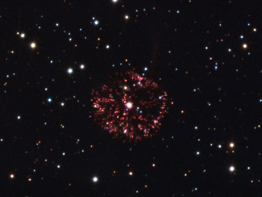
Composite optical image of the shell ejected by Nova GK Persei (1901), located 1500 light-years
away, as seen between 2003 and 2011. The shell contains about 10-4 Msun
and is about 1
light-year in diameter. Credit: Adam Block, Mt. Lemmon SkyCenter, University of Arizona; reproduced with permission.
- Movie_binaries:
Animation of mass transfer episodes in a compact binary system leading to
the explosion of the white dwarf/neutron star component
[Movie in preparation].
- Movie_nova115CO:
Time-evolution of the abundances in the innermost envelope
shell during a nova outburst on a 1.15 Msun CO accreting white dwarf,
as computed with the 1-D hydrodynamic code SHIVA.
- Movie_nova115ONe:
Time-evolution of the abundances in the innermost envelope
shell during a nova outburst on a 1.15 Msun ONe accreting white dwarf,
as computed with the 1-D hydrodynamic code SHIVA.
- Movie_nova135ONe:
Time-evolution of the abundances in the innermost envelope
shell during a nova outburst on a 1.35 Msun ONe accreting white dwarf,
as computed with the 1-D hydrodynamic code SHIVA.
- Movie_3Dmix_1:
Movie showing the onset of Kelvin–Helmholtz instabilities (t = 138 s - 325 s)
at the core-envelope interface during a nova outburst, in terms of the 12C mass
fraction, as computed in 3-D with the hydrodynamic code FLASH.
- Movie_3Dmix_2:
Movie showing the progress of Kelvin–Helmholtz instabilities (t = 339 s - 354 s)
at the core-envelope interface during a nova outburst, in terms of the 12C mass
fraction, as computed in 3-D with the hydrodynamic code FLASH.
Chapter 5: Type Ia Supernovae
- Fig5_1:
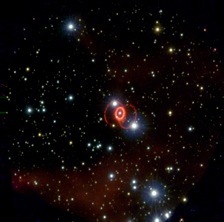
Composite image of the SN 1006 remnant, likely a type Ia supernova, located at 7100 light-years from Earth. The object is 65 light-years accross. Data has been obtained from NASA’s Chandra X-ray Observatory (X-rays), the University of Michigan’s 0.9 m Curtis Schmidt telescope at the NSF’s Cerro Tololo Inter-American Observatory (optical), the Digitized Sky Survey (optical), NRAO’s Very Large Array and Green Bank Telescope (radio). Credit: X-ray: NASA/CXC/Rutgers/G. Cassam-Chenaï, J. Hughes et al.; Radio: NRAO/AUI/NSF/GBT/VLA/Dyer, Maddalena, and Cornwell; Optical: Middlebury College/F. Winkler, NOAO/AURA/NSF/CTIO Schmidt and DSS; reproduced with permission.
- Fig5_2:
Composite image of the Crab nebula, the remnant of a type II supernova explosion, as
seen by NASA’s Hubble Space Telescope in 1999–2000. This six light-year wide object,
located 6500 light-years away, is composed of different chemical species, including neutral oxygen, singly ionized sulfur, hydrogen, and doubly ionized oxygen. The rapidly rotating neutron star embedded in the nebula acts as a dynamo, powering the nebula’s
interior glow (caused by electrons moving at nearly the speed of light around magnetic field lines of the compact star). Credit: NASA, ESA, J. Hester and A. Loll (Arizona State University). Source: http://hubblesite.org/gallery/album/pr2005037a/,
released into public domain by NASA.
- Fig5_3b:
Mosaic of the constellation Cassiopeia from NASA’s Wide-Field Infrared Survey Explorer (WISE), spanning an area of 1.6 × 1.6 degrees on the sky. Tychos’s supernova is the circular, nebular object in the upper left corner. Credit: NASA/JPL-Caltech. Source: http://commons.wikimedia.org/wiki/File:SN_1572_Tycho%27s_Supernova.jpg, released into public domain by NASA.
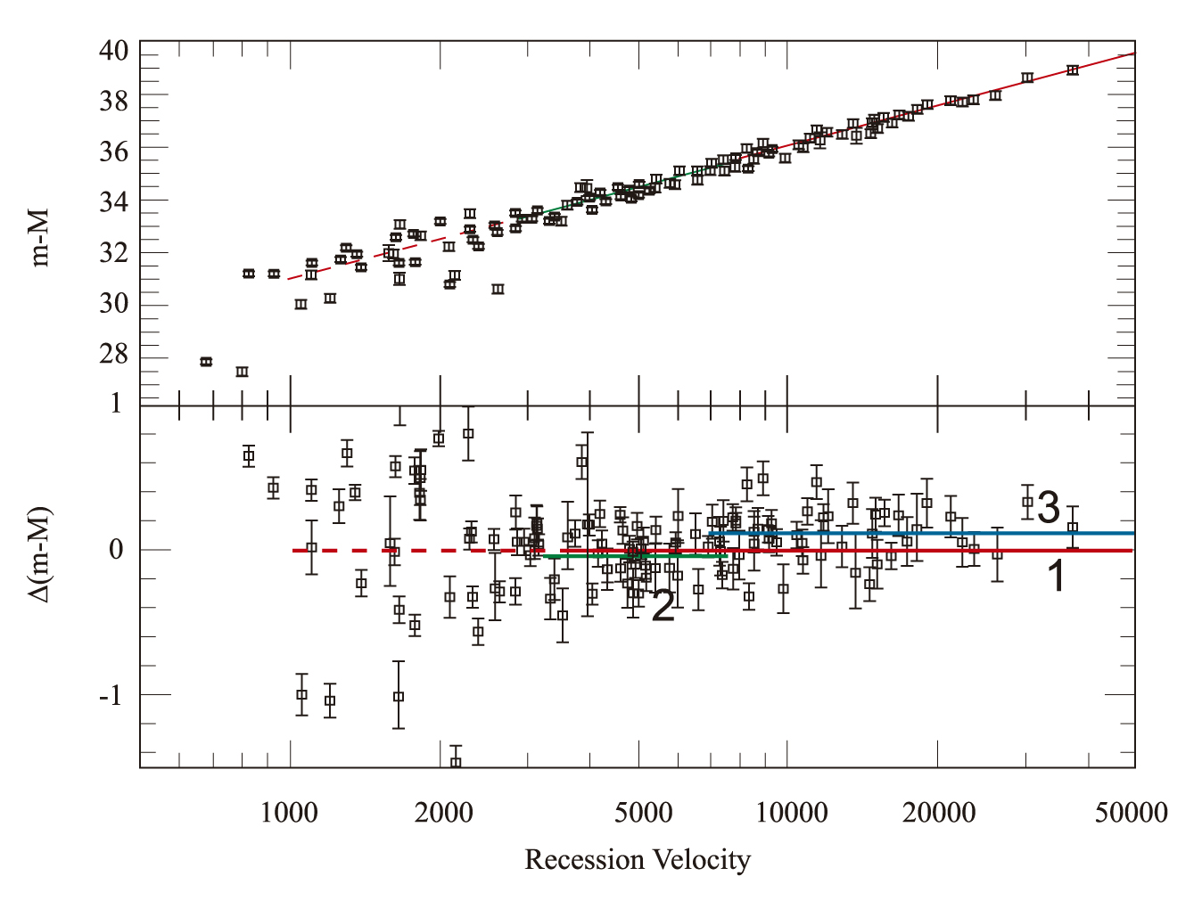
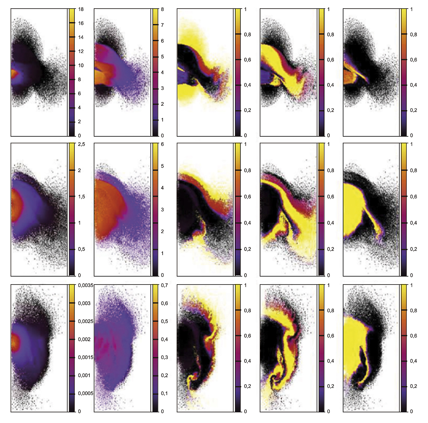
- Fig5_10:
Distribution of chemical species in the inner regions of an exploding white dwarf, for a
pure deflagration model (d) and two delayed-detonation models (a, c). Figure from Gamezo, Khokhlov, and Oran (2005); reproduced with permission.
- Fig5_12:
(Top) Hubble diagram of nearby type Ia supernovae depicting distance moduli (derived
from light curve shape corrected luminosities) vs. recession velocities (in km s-1, corrected to the rest frame of the cosmic microwave background, CMB). Fits to different recession
velocity ranges are also shown: v > 3000 km s-1 (1), 3000 km s-1 < v < 8000 km s-1 (2),
and v > 8000 km s-1 (3). (Bottom) Dispersion in distance moduli after substraction of the
expansion field from the data shown in the upper panel. Figure from Leibundgut (2008),
based on data from Jha et al. (2007); reproduced with permission.
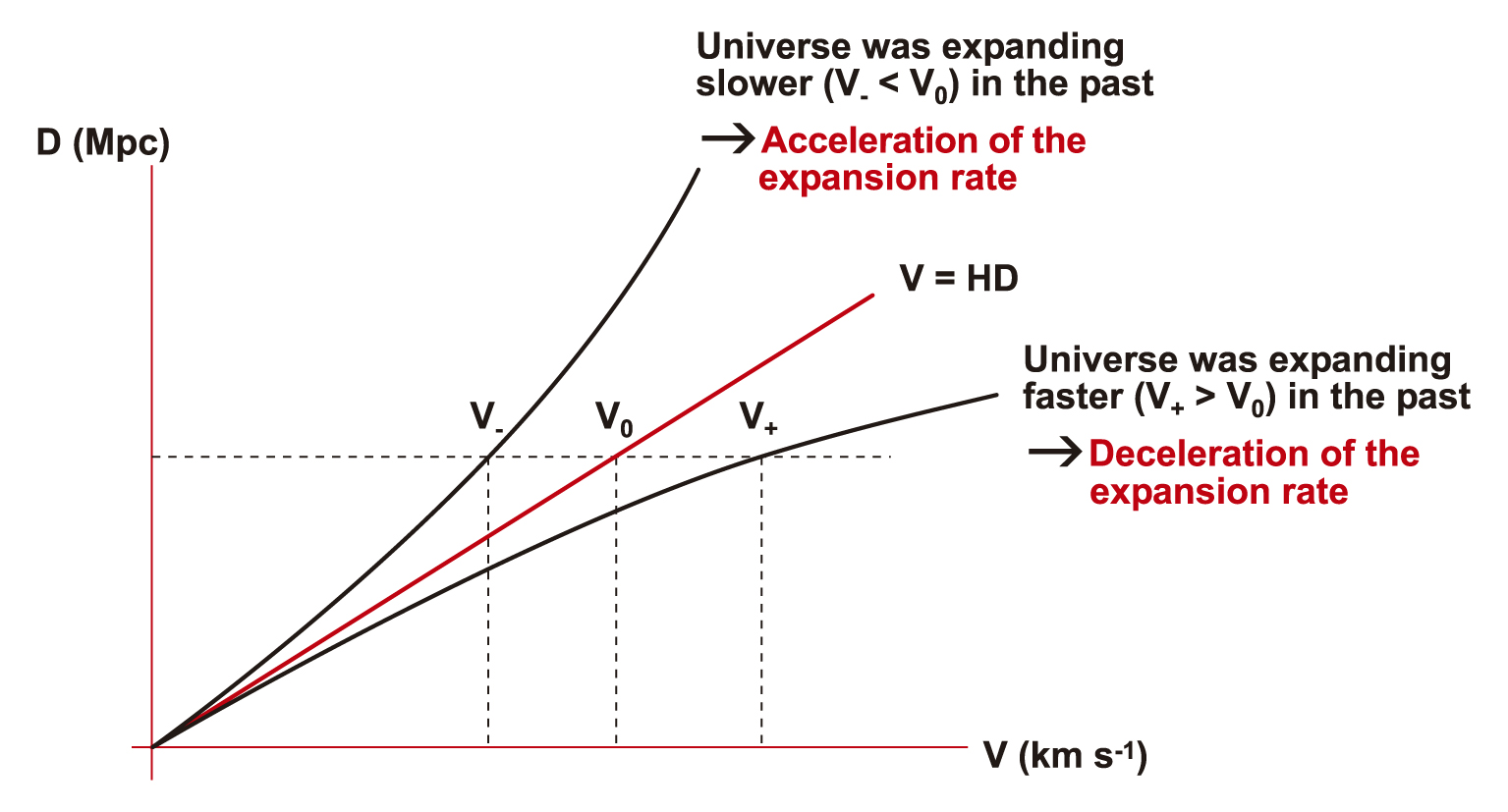
- Fig5_13:
Expansion rates in three possible models of the universe. Measurements at low redshifts (low
recession velocities) are in agreement with Hubble’s law, V = Ho D. If the expansion rate
has always been the same, all objects will follow a linear fit in a Hubble diagram, regardless
of their redshift (central line). In a universe now slowing its expansion rate (and therefore
characterized by a faster expansion in the past), an object at given distance D would show a
velocity larger than Ho D. Conversely, in a universe now speeding up, an object at distance D would show a velocity smaller than Ho D.
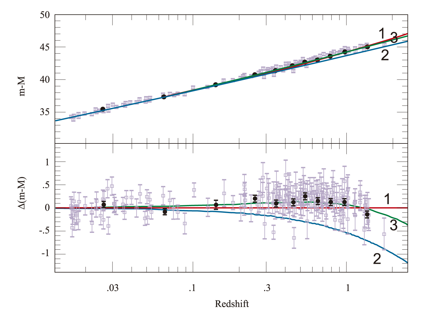
- Fig5_14:
(Top) Hubble diagram of distant type Ia supernovae, showing distance moduli (derived
from light curve shape corrected luminosities) vs. redshift (corrected to the rest frame of
the cosmic microwave background). Results assuming different model universes are shown
for comparison: (1) an empty universe (ΩΛ =
Ωm = 0); (2) the Einstein–de Sitter model
(ΩΛ = 0, Ωm = 1);
(3) best fit to data, corresponding to
ΩΛ = 0.7 and Ωm = 0.3.
(Bottom) Dispersion in distance moduli after substraction of the expansion field from
the data shown in the upper panel. Figure from Leibundgut (2008), based on data from
Davis et al. (2007); reproduced with permission.
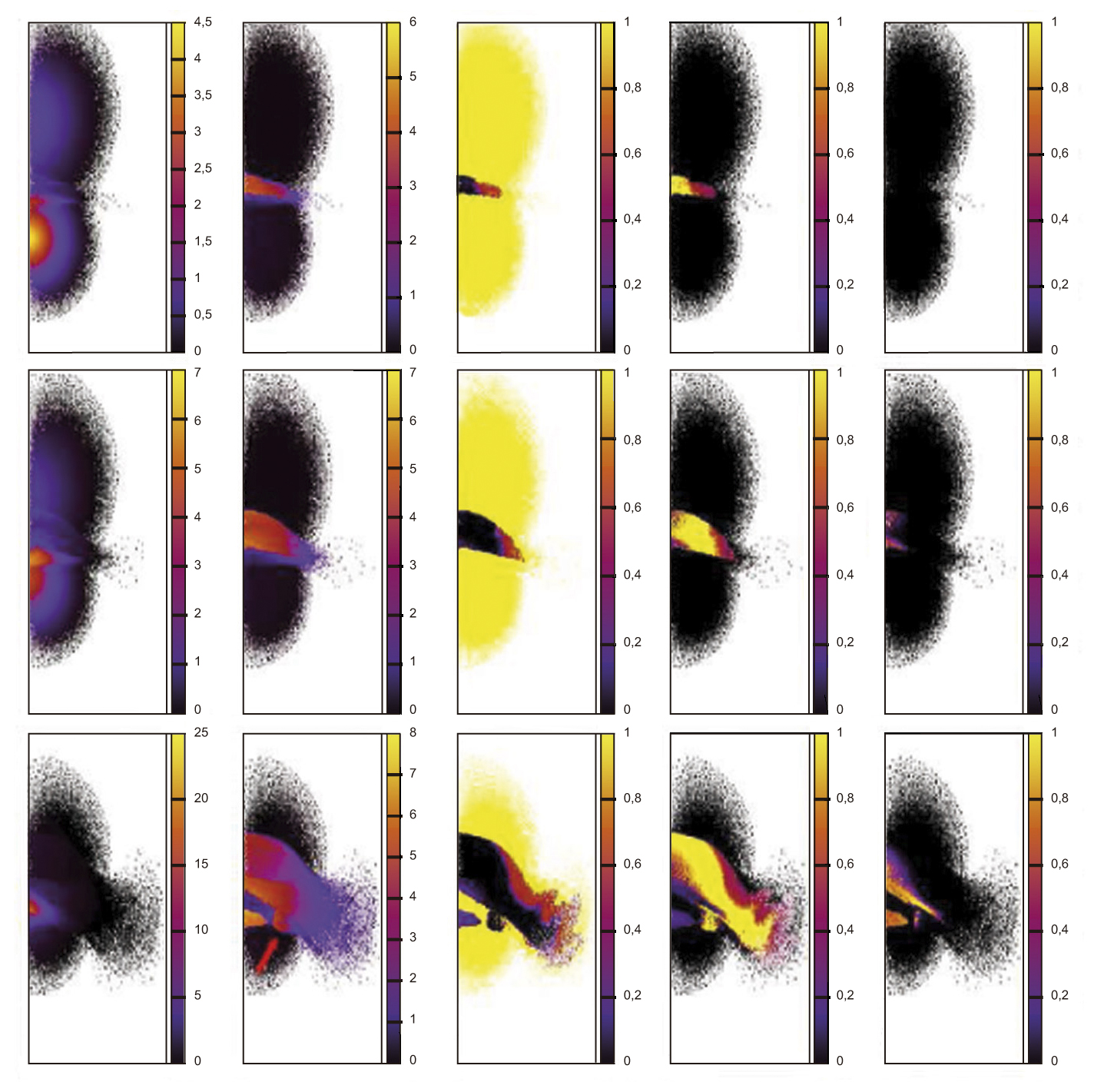
- Fig5_16 and
Fig5_17:
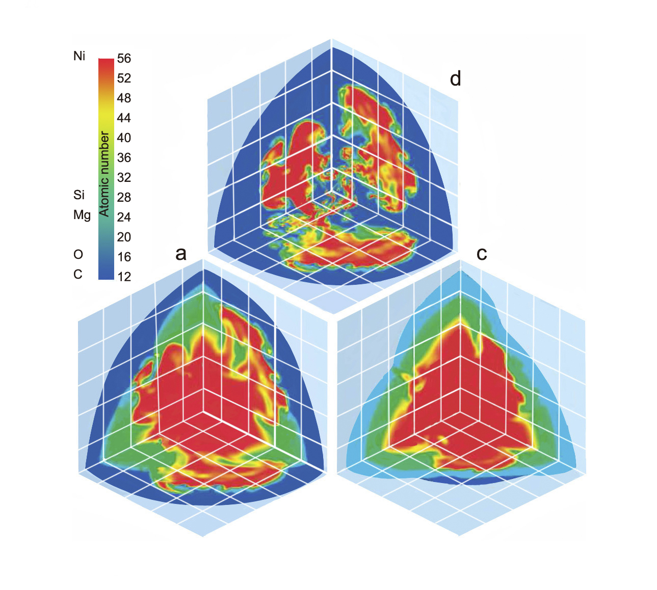
Snapshots of the evolution of a head-on collision of two CO white dwarfs, of masses
1.0 Msun and 0.81 Msun, resulting in a (super-Chandrasekhar) supernova explosion with an overall 56Ni
production of 1.02 Msun. Panels show, left to right, the density (in units of
107 g cm-3), temperature (109 K), and the mass fractions of
4He + 12C +16O, intermediate-mass elements
(20Ne to 40Ca), and Fe-group elements (44Ti to 60Zn), at different times since the beginning
of the simulation (from top to bottom, t = 16.9, 17.1, and 17.5 s [fig5_16] and
t = 17.6, 17.9, and 21.7 s [fig5_17]).
The simulation was performed in 2D with the axisymmetric SPH code AxisSPH using 88,560 particles.
Figures from Garcia-Senz et al. (2013); reproduced with permission.
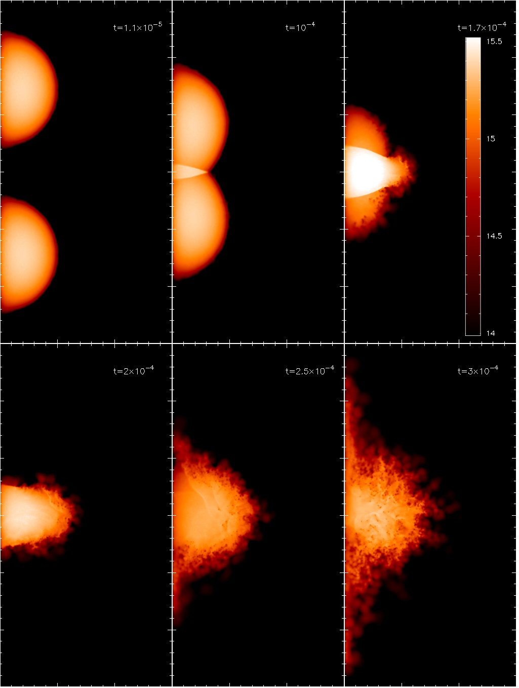
- Fig5_18:
Snapshots of the merging episode of two white dwarfs of masses
1.2 Msun and 0.4 Msun, simulated
with a smoothed-particle hydrodynamics code. Each panel shows the equatorial temperature contours as well as the location of the SPH particles. When the first particles of the
secondary star hit the surface of the primary (top right panel), the shocked regions reach
T = 5 × 10⁸ K. The colliding particles are reflected almost instantaneously by the hard
boundary of the primary. As mass transfer proceeds (central panels) the accreted matter
is shocked and heated on top of the surface of the primary. This matter is actually ejected
and a hot toroidal structure forms (right middle panel). Temperatures exceed 109 K, and
nuclear reactions transform the accreted He into C and O. Figure from Guerrero,
García-Berro and Isern (2004); reproduced with permission.
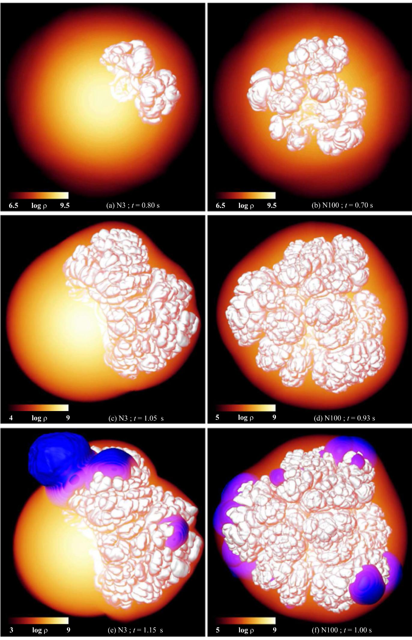
- Fig5_31: Snapshots of the evolution of two Chandrasekhar-mass, delayed detonation
models, with 3 ignition points (left panels) and 100 ignition points (right
panels). Figure from Seitenzahl et al. (2013).
Chapter 6: X-Ray Bursts and Superbursts
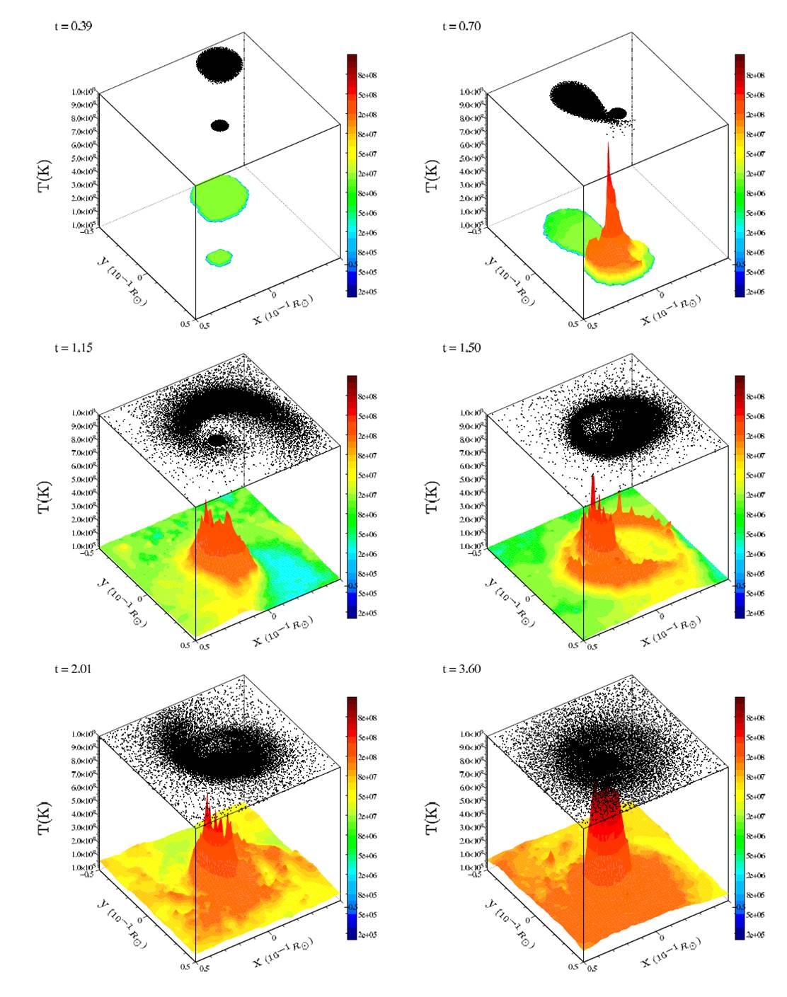
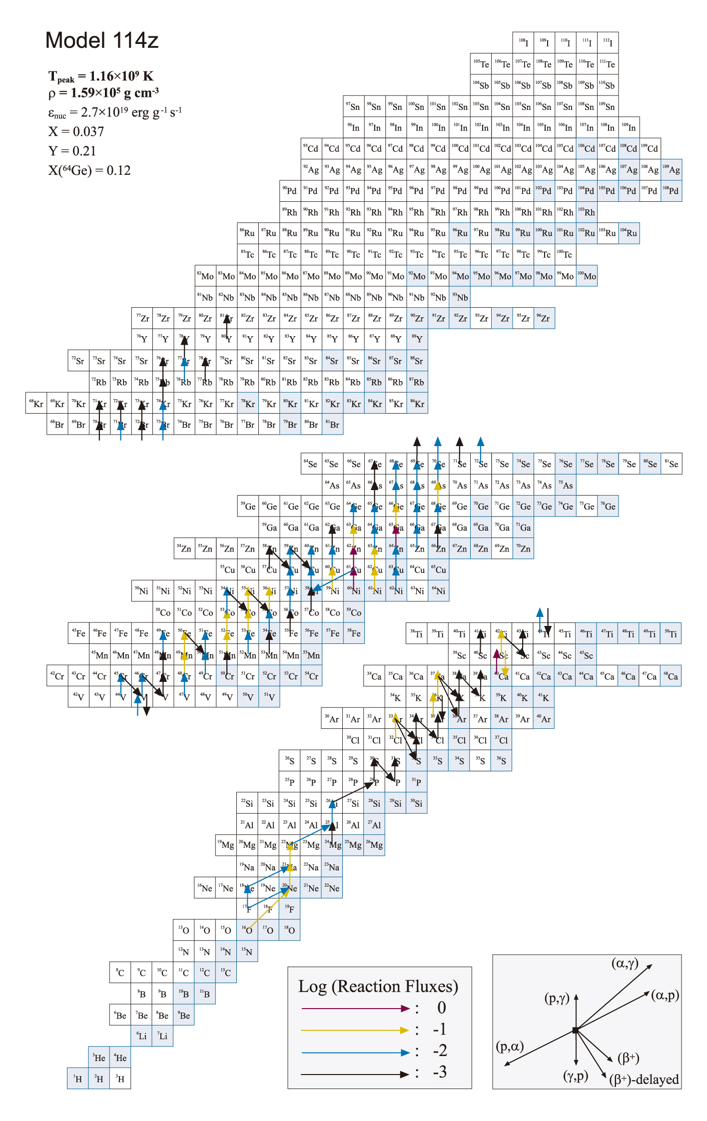
- Fig6_10:
Main reaction fluxes at the innermost envelope shell for Model 114z, at peak temperature
(Tbase,max = 1.16 × 10⁹ K), for the first computed burst.
Calculations have been performed
with the code SHIVA, and rely on a 1.4 Msun neutron star
(Lini = 1.6 × 1034 erg s-1 = 4.14
Lsun), accreting mass at a rate Macc = 1.8 × 10⁻⁹
Msun yr-1 (0.08 MEdd). The composition of
the accreted material is assumed to be solar-like (X = 0.7048, Y = 0.2752, Z = 0.02).
- Fig6_11:
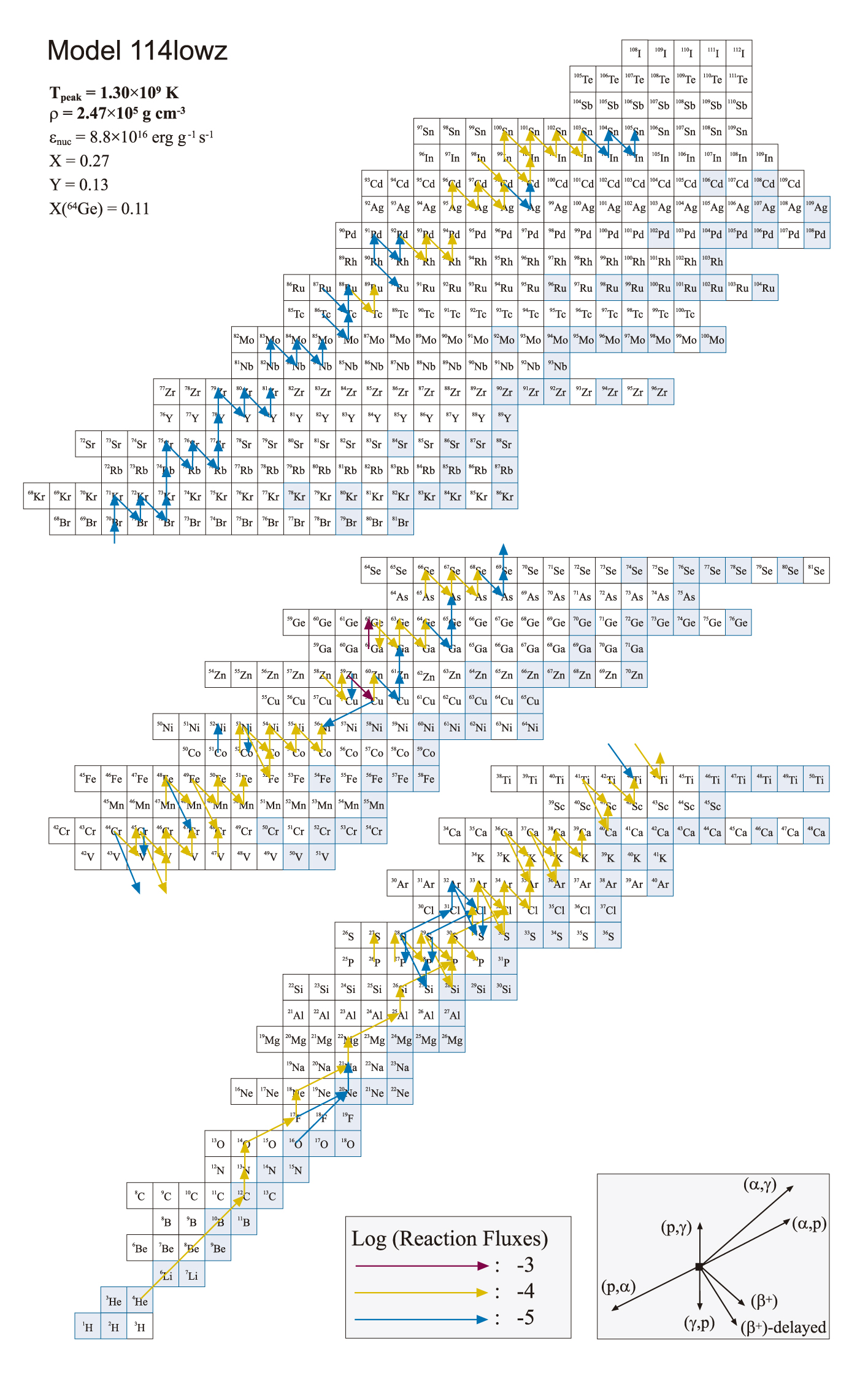
Main reaction fluxes at the innermost envelope shell for Model 114lowz, at peak temperature
(Tbase,max = 1.30 × 10⁹ K), for the first computed burst.
Calculations have been performed
with the code SHIVA, and rely on a 1.4 Msun neutron star
(Lini = 1.6 × 1034 erg s-1 = 4.14
Lsun), accreting mass at a rate Macc = 1.8 × 10⁻⁹
Msun yr-1 (0.08 MEdd). The composition of
the accreted material is assumed to be metal-poor (i.e., X = 0.759, Y = 0.240, and
Z = 0.001 = Zsun/20).
- Fig6_12:
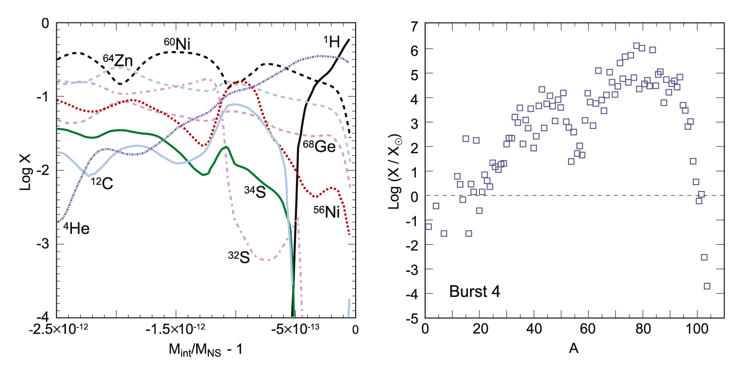
(Left panel) Mass fractions of the most abundant, stable isotopes (or with half-lifes > 1
hr) after 4 mixed H/He bursts, in Model 114z. (Right panel) Same as in
left panel, for overproduction factors with respect to solar abundances.
Figures adapted from José et al. (2010); reproduced with permission
- Fig6_15:
Example of sensitivity of a type I X-ray burst light curve to different choices of the
15O(α, γ) reaction rate: (panel 1) upper limit; (2) nominal rate; (3a to 3f)
lower limit, with different resolutions [75, 103, 129, 154, and 175 numerical shells, respectively].
Figure adapted from Fisker et al. (2006); reproduced with permission
[Figure in preparation].
- Fig6_16:
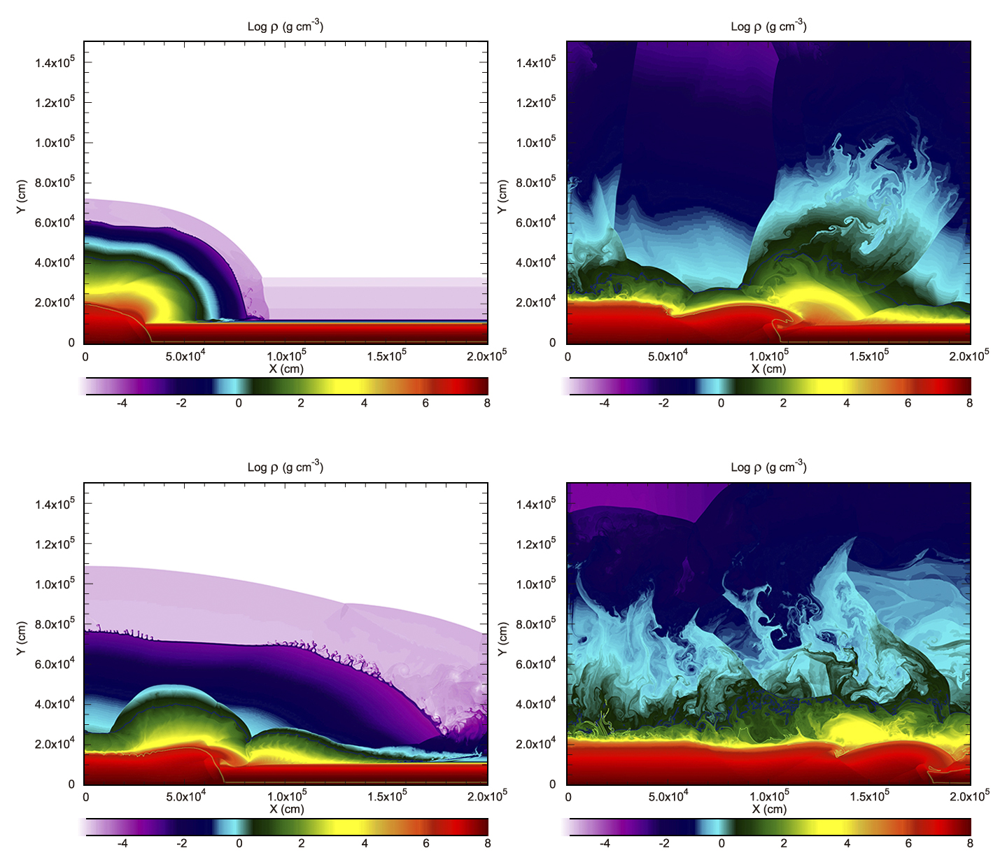
Snapshots of the propagation of a detonation front in a He-pure envelope on top of a neutron
star. Panels depict a density map at times 30 μs (upper left), 60 μs (lower left), 90 μs
(upper right), and 150 μs (lower right) since the onset of the detonation. Figure
adapted from Zingale et al. (2001); reproduced with permission.
- Movie_xrb_solar:
Time-evolution of the abundances in the innermost envelope
shell during a type I X-ray burst driven by accretion of solar composition material onto
a 1.44 Msun neutron star, as computed with the 1-D hydrodynamic code SHIVA.
- Movie_xrb_lowz:
Time-evolution of the abundances in the innermost envelope
shell during a type I X-ray burst driven by accretion of low metallicity material onto
a 1.44 Msun neutron star, as computed with the 1-D hydrodynamic code SHIVA.
Chapter 7: Core-Collapse Supernovae
- Fig7_1:
SN 1987A, the closest supernova detected since the invention of the telescope.
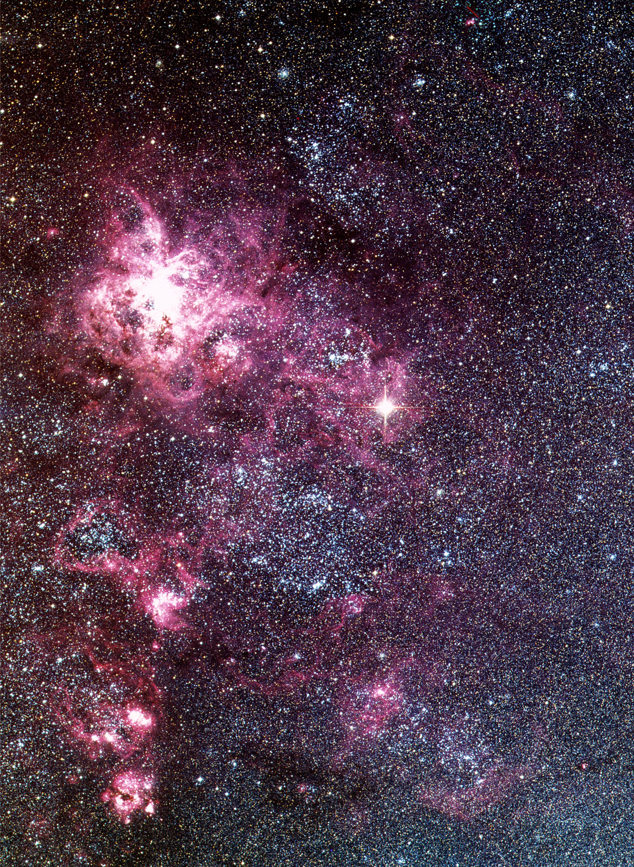
The object corresponds to the very bright star in the middle right of the Tarantula Nebula, in the Large Magellanic Cloud. At the time of this picture, SN 1987A was visible with the naked eye.
Credit: ESO. Source: http://www.eso.org/public/images/eso0708a/; released into public domain by ESO.
- Fig7_2:
Glowing gas rings surrounding SN 1987A, as seen by the Hubble Space Telescope in February 1994. Credit: P. Challis, Harvard–Smithsonian Center for Astrophysics.
Source: http://hubblesite.org/newscenter/archive/releases/1998/
08/image/g/; released into public domain by NASA.
- Fig7_11:
Time-evolution of the density during the head-on collision of two neutron stars. Calculations were performed in 2D with an SPH code. Figure courtesy of R. Cabezón
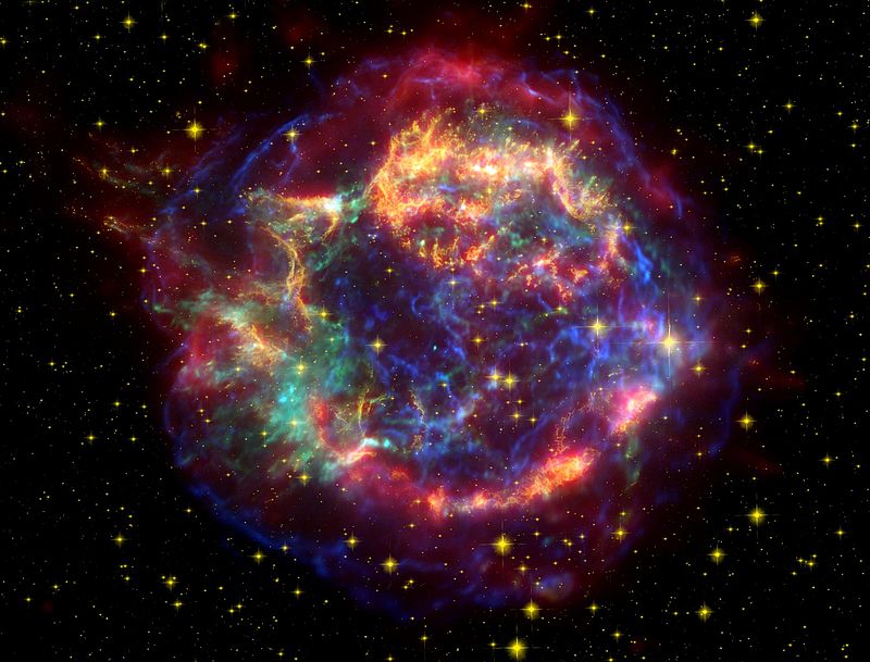
- Fig7_13:
Composite image of the supernova remnant Cassiopeia A (Cas A), based on observations from Hubble and Spitzer telescopes as well as Chandra X-ray Observatory. While Spitzer has mapped the distribution of warm dust (about 100 K) in the outer shells, Hubble has revealed filamentary structures of hot plasma (10,000 K), and Chandra has imaged the distribution of very hot plasma (T = 107 K) created in the collision between the
ejecta and the surrounding gas and dust. Moreover, Chandra has also spotted the
neutron star located near the center of Cassiopeia A’s remnant.
Credit: NASA/JPL–Caltech/O. Krause (Steward Observatory). Source:
http://www.spitzer.caltech.edu/images/1445-ssc2005-14c-Cassiopeia-A-Death-Becomes-Her; released into public domain by NASA.
- Fig7_15:
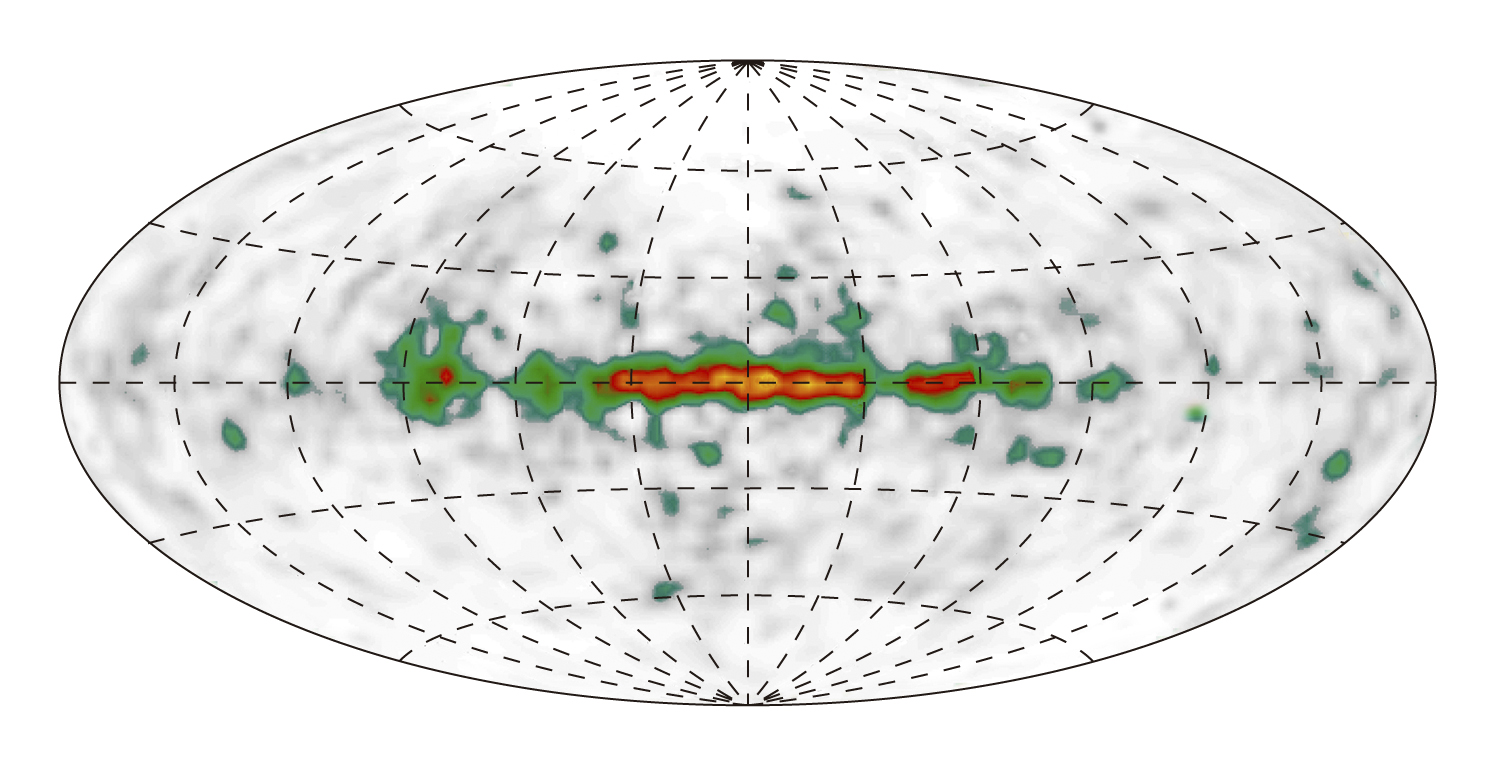
Maximum entropy, all-sky map of the Galactic 26Al 1.809 MeV emission observed with the COMPTEL instrument on board CGRO satellite over 9 years.
Figure adapted from Plüschke et al. (2001); reproduced with permission.
- Fig7_16:
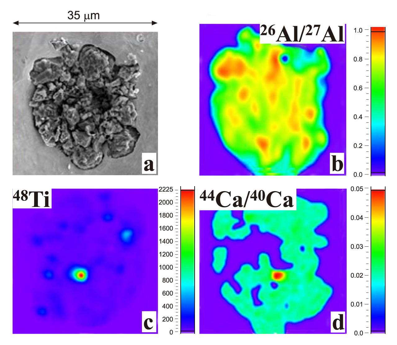
SEM image (panel a) and NanoSIMS isotopic maps of 26Al/27Al, 48Ti, and 44Ca/40Ca
(panels b, c, and d) of an unusually large (about 30 μm) SiC grain of type X named Bonanza. The SEM image suggests that the grain is actually an aggregate of smaller grains. The anomalous
size of Bonanza has allowed the determination of isotopic ratios for many different elements,
including Li, B, C, N, Al-Mg, Si, S, Ca, Ti, Fe, and Ni. Isotopic analyses yield
12C/13C = 190,
14N/15N = 28,
δ29Si/28Si = -282‰, and
δ30Si/28Si = -442‰. Mg is
completely dominated by the presence of radiogenic 26Mg, from the decay of 26Al (the ratio 26Al/27Al inferred in the grain lays in the range 0.4 – 0.9). The region with the largest 44Ca/40Ca ratio (0.05), corresponds to a titanium subgrain, which exhibits as well the largest concentration of 48Ti. This suggests that the 44Ca excess corresponds to in situ decay of 44Ti. The Ti, Fe, and Ni isotopic patterns are typical of other X grains and can be reproduced by mixing different layers in models of core-collapse supernovae. Figure adapted from Zinner et al. (2011); reproduced with permission.
- Fig7_18:
Evolution of the density and magnetic field during the merging of a binary neutron star
system, at four different times (t = 7.4 ms, 13.8 ms, 15.3 ms, and 26.5 ms). The simulation yields a rapidly spinning black hole surrounded by a hot and highly magnetized torus. Magnetohydrodynamical instabilities can actually amplify an initially turbulent magnetic field along the black hole spin axis, naturally resulting in a relativistic jet, potentially powering a short GRB. Figure from Rezzolla et al.
(2011); reproduced with permission.
Appendix 2: Computer Program for the Free-Fall Collapse
Problem
- freefall.f: 1-D hydrocode (in Fortran)
for the simulation of the free-fall collapse of a homogeneous sphere.
- FREE.INI: Input file for freefall.f.
SOLUTIONS MANUAL
Back to Home
Page